flowcatchR: A framework for tracking and analyzing flowing blood cells in time lapse microscopy images
Federico Marini
Institute of Medical Biostatistics, Epidemiology and Informatics (IMBEI), MainzCenter for Thrombosis and Hemostasis (CTH), Mainzmarinif@uni-mainz.de
Johanna Mazur
Institute of Medical Biostatistics, Epidemiology and Informatics (IMBEI), MainzHarald Binder
Institute of Medical Biostatistics, Epidemiology and Informatics (IMBEI), Mainz1 December 2025
Source:vignettes/flowcatchr_vignette.Rmd
flowcatchr_vignette.RmdAbstract
flowcatchR is a set of tools to analyze in vivo microscopy imaging data, focused on tracking flowing blood cells. flowcatchR guides throughout all the steps of bioimage processing, from segmentation to calculation of features, filtering out particles not of interest, providing also a set of utilities to help checking the quality of the performed operations. The main novel contribution investigates the issue of tracking flowing cells such as the ones in blood vessels, to categorize the particles in flowing, rolling, and adherent by providing a comprehensive analysis of the identified trajectories. The extracted information is then applied in the study of phenomena such as hemostasis and thrombosis development. We expect this package to be potentially applied to a variety of assays, covering a wide range of applications founded on time-lapse microscopy.
Compiled date: 2025-12-01
Last edited: 2018-01-14
License: BSD_3_clause + file LICENSE
Introduction
This document offers an introduction and overview of the R/Bioconductor Gentleman et al. (2004) package flowcatchR, which provides a flexible and comprehensive set of tools to detect and track flowing blood cells in time-lapse microscopy.
Why flowcatchR?
flowcatchR builds upon functionalities provided by the EBImage package (Pau et al. 2010), and extends them in order to analyze time-lapse microscopy images. Here we list some of the unique characteristics of the datasets flowcatchR is designed for:
- The images come from intravital microscopy experiments. This means that the Signal-to-Noise Ratio (SNR) is not optimal, and, very importantly, there are potential major movements of the living specimen that can be confounded with the true movements of the particles of interest (Meijering and Smal 2008)
- Cells are densely distributed on the images, with particles that can enter and leave the field of view
- The acquisition frame rate is a compromise between allowing the fluorescent cells to be detected and detecting the movements properly
- Cells can flow, temporarily adhere to the endothelial layer and/or be permanently adherent. Therefore, all movement modalities should be detected correctly throughout the entire acquisition. Cells can also cluster together and form (temporary) conglomerates
Essential features flowcatchR delivers to the user are:
- A simple and flexible, yet complete framework to analyze flowing
blood cells (and more generally time-lapse) image sets, with a system of
S4 classes such as
Frames,ParticleSet, andTrajectorySetconstituting the backbone of the procedures - Techniques for aiding the detection of objects in the segmentation step
- An algorithm for tracking the particles, adapted and improved from the proposal of Sbalzarini and Koumoutsakos (2005) (Sbalzarini and Koumoutsakos 2005), that reflects the directional aspect of the motion
- A wide set of functions inspecting the kinematic properties of the identified trajectories Meijering, Dzyubachyk, and Smal (2012), providing publication-ready summary statistics and visualization tools to help classifying identified objects
This guide includes a brief overview of the entire processing flow, from importing the raw images to the analysis of kinematic parameters derived from the identified trajectories. An example dataset will be used to illustrate the available features, in order to track blood platelets in consecutive frames derived from an intravital microscopy acquisition (also available in the package). All steps will be dissected to explore available parameters and options.
Purpose of this document
This vignette includes a brief overview of the entire processing flow, from importing the raw images to the analysis of kinematic parameters derived from the identified trajectories. An example dataset will be used to illustrate the available features, in order to track blood platelets in consecutive frames derived from an intravital microscopy acquisition (also available in the package). All steps will be dissected to explore available parameters and options.
Getting started
Installation
flowcatchR is an R package distributed as part of the Bioconductor project. To install flowcatchR, please start R and type:
if (!requireNamespace("BiocManager", quietly=TRUE))
    install.packages("BiocManager")
BiocManager::install("flowcatchR")
In case you might prefer to install the latest development version, this can be done with these two lines below:
install.packages("devtools") # if needed
devtools::install_github("federicomarini/flowcatchR")
Installation issues should be reported to the Bioconductor support site (http://support.bioconductor.org/).
Getting help
The flowcatchR
package was tested on a variety of datasets provided from cooperation
partners, yet it may require some extra tuning or bug fixes. For these
issues, please contact the maintainer - if required with a copy of the
error messages, the output of sessionInfo function:
maintainer("flowcatchR")## [1] "Federico Marini <marinif@uni-mainz.de>"Despite our best efforts to test and develop the package further, additional functions or interesting suggestions might come from the specific scenarios that the package users might be facing. Improvements of existing functions or development of new ones are always most welcome! We also encourage to fork the GitHub repository of the package (https://github.com/federicomarini/flowcatchR), develop and test the new feature(s), and finally generate a pull request to integrate it to the original repository.
Citing flowcatchR
The work underlying the development of flowcatchR
has not been formally published yet. A manuscript has been submitted for
peer-review. For the time being, users of flowcatchR
are encouraged to cite it using the output of the citation
function, as it follows:
citation("flowcatchR")## To cite the package 'flowcatchR' in publications use:
##
## Federico Marini, Harald Binder (2018). flowcatchR: Tools to analyze
## in vivo microscopy imaging data focused on tracking flowing blood
## cells. URL http://bioconductor.org/packages/flowcatchR/ doi:
## 10.18129/B9.bioc.flowcatchR
##
## A BibTeX entry for LaTeX users is
##
## @Manual{,
## title = {{flowcatchR}: Tools to analyze in vivo microscopy imaging data focused on
## tracking flowing blood cells},
## author = {Federico Marini and Harald Binder},
## year = {2018},
## url = {http://bioconductor.org/packages/flowcatchR/},
## doi = {10.18129/B9.bioc.flowcatchR},
## }Processing overview
flowcatchR works primarily with sets of fluorescent time-lapse images, where the particles of interest are marked with a fluorescent label (e.g., red for blood platelets, green for leukocytes). Although different entry spots are provided (such as the coordinates of identified points in each frame via tab delimited files), we will illustrate the characteristics of the package starting from the common protocol starting point. In this case, we have a set of 20 frames derived from an intravital microscopy acquisition, which for the sake of practicality were already registered to reduce the unwanted specimen movements (Fiji (Schindelin, Arganda-Carreras, and Frise 2012) was used for this purpose).
## Loading required package: EBImage
data("MesenteriumSubset")
# printing summary information for the MesenteriumSubset object
MesenteriumSubset
## Frames
## colorMode : Color
## storage.mode : double
## dim : 271 131 3 20
## frames.total : 60
## frames.render: 20
##
## imageData(object)[1:5,1:6,1,1]
## [,1] [,2] [,3] [,4] [,5] [,6]
## [1,] 0.1647059 0.2117647 0.1882353 0.1803922 0.1607843 0.1333333
## [2,] 0.2352941 0.1882353 0.1803922 0.1568627 0.1411765 0.1372549
## [3,] 0.2352941 0.2000000 0.1764706 0.1490196 0.1333333 0.1333333
## [4,] 0.2352941 0.2117647 0.1764706 0.1529412 0.1411765 0.1411765
## [5,] 0.2313725 0.2078431 0.1725490 0.1411765 0.1294118 0.1411765
##
## Channel(s): allTo obtain the set of trajectories identified from the analysis of the loaded frames, a very compact one-line command is all that is needed:
# one command to seize them all :)
fullResults <- kinematics(trajectories(particles(channel.Frames(MesenteriumSubset,"red"))))
On a MAC OS X machine equipped with 2.8 Ghz Intel Core i7 processor and 16 GB RAM, the execution of this command takes 2.32 seconds to run (tests performed with the R package microbenchmark. On a more recent MacBook Pro (2017), the same benchmark took 1.78 seconds.
The following sections will provide additional details to the operations mentioned above, with more also on the auxiliary functions that are available in flowcatchR.
Image acquisition
A set of images is acquired, after a proper microscopy setup has been performed. This includes for example a careful choice of spatial and temporal resolution; often a compromise must be met to have a good frame rate and a good SNR to detect the particles in the single frames. For a good review on the steps to be taken, please refer to Meijering’s work Meijering, Dzyubachyk, and Smal (2012).
flowcatchR
provides an S4 class that can store the information of a complete
acquisition, namely Frames. The Frames class
extends the Image class, defined in the EBImage
package, and thus exploits the multi-dimensional array structures of the
class. The locations of the images are stored as dimnames
of the Frames object. To construct a Frames
object from a set of images, the read.Frames function is
used:
# initialization
fullData <- read.Frames(image.files="/path/to/folder/containing/images/", nframes=100)
# printing summary information for the Frames object
fullData
nframes specifies the number of frames that will
constitute the Frames object, whereas
image.files is a vector of character strings with the full
location of the (raw) images, or the path to the folder containing them
(works automatically if images are in TIFF/JPG/PNG format). In this case
we just loaded the full dataset, but for the demonstrational purpose of
this vignette, we will proceed with the subset available in the
MesenteriumSubset object, which we previously loaded in
Section @ref(overview).
It is possible to inspect the images composing a Frames
object with the function inspect.Frames (Fig.
@ref(fig:inspectRaw)).
inspect.Frames(MesenteriumSubset, nframes=9, display.method="raster")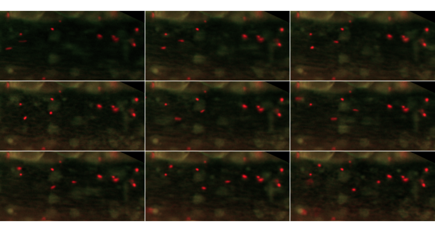
The first 9 frames of the MesenteriumSubset dataset. The red channel stores information about platelets, while the green channel is dedicated to leukocytes
By default, display.method is set to
browser, as in the EBImage
function display. This opens up a window in the predefined browser
(e.g. Mozilla Firefox), with navigable frames (arrows on the top left
corner). For the vignette, we will set it to raster, for
viewing them as raster graphics using R’s native functions.
Importantly, these image sets were already registered and rotated in such a way that the overall direction of the movement of interest flows from left to right, as a visual aid and also to fit with some assumptions that will be done in the subsequent step of particle tracking. To register the images, we recommend the general purpose tools offered by suites such as ImageJ/Fiji Schindelin, Arganda-Carreras, and Frise (2012).
For the following steps, we will focus on the information contained
in the red channel, corresponding in this case to blood platelets. We do
so by calling the channel.Frames function:
plateletsMesenterium <- channel.Frames(MesenteriumSubset, mode="red")
plateletsMesenterium
## Frames
## colorMode : Grayscale
## storage.mode : double
## dim : 271 131 20
## frames.total : 20
## frames.render: 20
##
## imageData(object)[1:5,1:6,1]
## [,1] [,2] [,3] [,4] [,5] [,6]
## [1,] 0.1647059 0.2117647 0.1882353 0.1803922 0.1607843 0.1333333
## [2,] 0.2352941 0.1882353 0.1803922 0.1568627 0.1411765 0.1372549
## [3,] 0.2352941 0.2000000 0.1764706 0.1490196 0.1333333 0.1333333
## [4,] 0.2352941 0.2117647 0.1764706 0.1529412 0.1411765 0.1411765
## [5,] 0.2313725 0.2078431 0.1725490 0.1411765 0.1294118 0.1411765
##
## Channel(s): redThis creates another instance of the class Frames, and
we inspect it in its first 9 frames
(Fig.@ref(fig:inspectPlatelets)).
inspect.Frames(plateletsMesenterium, nframes=9, display.method="raster")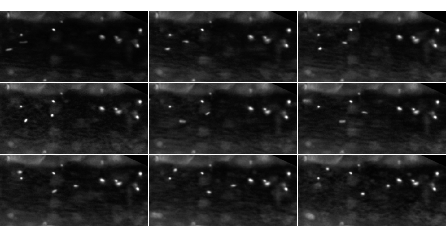
The first 9 frames for the red channel of the MesenteriumSubset dataset.
This is just displaying the GrayScale signal for the red channel stored
in plateletsMesenterium (for the thrombocytes)
Image preprocessing and analysis
Steps such as denoising, smoothing and morphological operations
(erosion/dilation, opening/closing) can be performed thanks to the
general functions provided by EBImage.
flowcatchR
offers a wrapper around a series of operations to be applied to all
images in a Frames object. The function
preprocess.Frames is called via the following command:
preprocessedPlatelets <- preprocess.Frames(plateletsMesenterium,
                                    brush.size=3, brush.shape="disc",
                                    at.offset=0.15, at.wwidth=10, at.wheight=10,
                                    kern.size=3, kern.shape="disc",
                                    ws.tolerance=1, ws.radius=1)
preprocessedPlatelets
## Frames
## colorMode : Grayscale
## storage.mode : integer
## dim : 271 131 20
## frames.total : 20
## frames.render: 20
##
## imageData(object)[1:5,1:6,1]
## [,1] [,2] [,3] [,4] [,5] [,6]
## [1,] 0 0 0 0 0 0
## [2,] 0 0 0 0 0 0
## [3,] 0 0 0 0 0 0
## [4,] 0 0 0 0 0 0
## [5,] 0 0 0 0 0 0
##
## Channel(s): redThe result of this is displayed in Fig.@ref(fig:inspectSegm). For a
detailed explanation of the parameters to better tweak the performances
of this segmentation step, please refer to the help of
preprocess.Frames. To obtain an immediate feedback about
the effects of the operations performed in the full preprocessing phase,
we can call again inspect.Frames on the Frames
of segmented images (Fig.@ref(fig:inspectSegm).
inspect.Frames(preprocessedPlatelets, nframes=9, display.method="raster")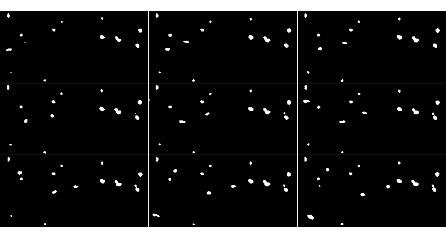
The first 9 frames after preprocessing of the MesenteriumSubset dataset. The binarized image shows the detected objects after thresholding.
The frames could be cropped, if e.g. it is needed to remove
background noise that might be present close to the edges. This is done
with the function crop.Frames.
croppedFrames <- crop.Frames(plateletsMesenterium,
                     cutLeft=6, cutRight=6,
                     cutUp=3, cutDown=3,
                     testing=FALSE)
croppedFrames
## Frames
## colorMode : Grayscale
## storage.mode : double
## dim : 260 126 20
## frames.total : 20
## frames.render: 20
##
## imageData(object)[1:5,1:6,1]
## [,1] [,2] [,3] [,4] [,5] [,6]
## [1,] 0.1803922 0.1568627 0.1372549 0.1372549 0.1333333 0.1176471
## [2,] 0.2039216 0.1843137 0.1490196 0.1254902 0.1215686 0.1215686
## [3,] 0.1843137 0.1764706 0.1568627 0.1294118 0.1176471 0.1019608
## [4,] 0.1921569 0.1568627 0.1529412 0.1333333 0.1254902 0.1333333
## [5,] 0.2000000 0.1647059 0.1490196 0.1450980 0.1333333 0.1411765
##
## Channel(s): redIf testing is set to true, the function just displays
the first cropped frame, to get a feeling whether the choice of
parameters was adequate. Similarly, for the function
rotate.Frames the same behaviour is expected, whereas the
rotation in degrees is specified by the parameter
angle.
rotatedFrames <- rotate.Frames(plateletsMesenterium, angle=30)
rotatedFrames
## Frames
## colorMode : Grayscale
## storage.mode : double
## dim : 300 249 20
## frames.total : 20
## frames.render: 20
##
## imageData(object)[1:5,1:6,1]
## [,1] [,2] [,3] [,4] [,5] [,6]
## [1,] 0 0 0 0 0 0
## [2,] 0 0 0 0 0 0
## [3,] 0 0 0 0 0 0
## [4,] 0 0 0 0 0 0
## [5,] 0 0 0 0 0 0
##
## Channel(s): redIf desired, it is possible to select just a subset of the frames
belonging to a Frames. This can be done via the
select.Frames function:
subsetFrames <- select.Frames(plateletsMesenterium,
                       framesToKeep=c(1:10,14:20))
subsetFrames
## Frames
## colorMode : Grayscale
## storage.mode : double
## dim : 271 131 17
## frames.total : 17
## frames.render: 17
##
## imageData(object)[1:5,1:6,1]
## [,1] [,2] [,3] [,4] [,5] [,6]
## [1,] 0.1647059 0.2117647 0.1882353 0.1803922 0.1607843 0.1333333
## [2,] 0.2352941 0.1882353 0.1803922 0.1568627 0.1411765 0.1372549
## [3,] 0.2352941 0.2000000 0.1764706 0.1490196 0.1333333 0.1333333
## [4,] 0.2352941 0.2117647 0.1764706 0.1529412 0.1411765 0.1411765
## [5,] 0.2313725 0.2078431 0.1725490 0.1411765 0.1294118 0.1411765
##
## Channel(s): redIf required, the user can decide to perform a normalization step (via
normalizeFrames), to correct for systematic variations in
the acquisition conditions, in case the overall intensity levels change,
e.g., when the acquisition spans long time scales. In this case, the
median of the intensity sums is chosen as a scaling factor.
normFrames <- normalizeFrames(plateletsMesenterium,normFun = "median")The user can choose any combination of the operations in order to
segment the images provided as input, but preprocess.Frames
is a very convenient high level function for proceeding in the workflow.
It is also possible, as it was shown in the introductory one-liner, to
call just particles on the raw Frames object.
In this latter case, particles computes the preprocessed
Frames object according to default parameters. Still, in
either situation, the output for this step is an object of the
ParticleSet class.
platelets <- particles(plateletsMesenterium, preprocessedPlatelets)## Computing features in parallel...
## Done!
platelets## An object of the ParticleSet class.
##
## Set of particles for 20 images
##
## Displaying a subset of the features of the 13 particles found in the first image...
## cell.0.m.cx cell.0.m.cy cell.0.m.majoraxis cell.0.m.eccentricity
## 1 186.70833 47.937500 8.916405 0.6353715
## 2 256.19048 35.857143 7.746554 0.4606665
## 3 251.09524 63.523810 8.552466 0.6843186
## 4 215.54688 51.828125 13.694783 0.8788344
## 5 15.82759 8.517241 7.548790 0.7570114
## cell.0.m.theta cell.0.s.area cell.0.s.perimeter cell.0.s.radius.mean
## 1 0.3380463 48 20 3.487042
## 2 0.9165252 42 19 3.194559
## 3 0.9370618 42 19 3.247531
## 4 0.7172299 64 28 4.308530
## 5 1.5439842 29 16 2.622403
##
## Particles identified on the red channelThe function particles leverages on the multi-core
architecture of the systems where the analysis is run, and this is
implemented via BiocParallel
(updated since Version 1.0.3).
As it can be seen from the summary information, each
ParticleSet stores the essential information on all
particles that were detected in the original images, alongside with a
complete set of features, which are computed by integrating the
information from both the raw and the segmented frames.
A ParticleSet can be seen as a named list, where each
element is a data.frame for a single frame, and the image
source is stored as names to help backtracking the
operations performed, and the slot channel is retained as
selected in the initial steps.
It is possible to filter out particles according to their properties,
such as area, shape and eccentricity. This is possible with the function
select.particles. The current implementation regards only
the surface extension, but any additional feature can be chosen and
adopted to restrict the number of candidate particles according to
particular properties which are expected and/or to remove potential
noise that went through the preprocessing phase.
selectedPlatelets <- select.particles(platelets, min.area=3)## Filtering the particles...
selectedPlatelets## An object of the ParticleSet class.
##
## Set of particles for 20 images
##
## Displaying a subset of the features of the 13 particles found in the first image...
## cell.0.m.cx cell.0.m.cy cell.0.m.majoraxis cell.0.m.eccentricity
## 1 186.70833 47.937500 8.916405 0.6353715
## 2 256.19048 35.857143 7.746554 0.4606665
## 3 251.09524 63.523810 8.552466 0.6843186
## 4 215.54688 51.828125 13.694783 0.8788344
## 5 15.82759 8.517241 7.548790 0.7570114
## cell.0.m.theta cell.0.s.area cell.0.s.perimeter cell.0.s.radius.mean
## 1 0.3380463 48 20 3.487042
## 2 0.9165252 42 19 3.194559
## 3 0.9370618 42 19 3.247531
## 4 0.7172299 64 28 4.308530
## 5 1.5439842 29 16 2.622403
##
## Particles identified on the red channelThis step can be done iteratively, with the help of the function
add.contours. If called with the parameter
mode set to particles, then it will
automatically generate a Frames object, with the contours
of all particles drawn around the objects that passed the segmentation
(and filtering) step (Fig.@ref(fig:checkSelection)).
paintedPlatelets <- add.contours(raw.frames=MesenteriumSubset,
                                 binary.frames=preprocessedPlatelets,
                                 mode="particles")
inspect.Frames(paintedPlatelets, nframes=9, display.method="raster")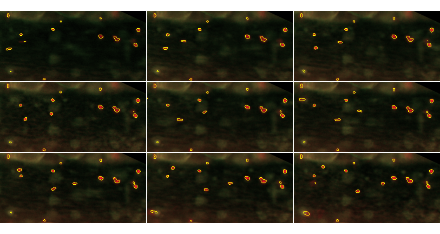
Particles detected in the first 9 frames. Particles detected in the first 9 frames are shown in yellow, with their contours defined by the segmentation procedure.
To connect the particles from one frame to the other, we perform first the detection of particles on all images. Only in a successive phase, we establish the links between the so identified objects. This topic will be covered in detail in the following section.
Particle tracking
To establish the connections between particles, the function to be
called is link.particles. The algorithm used to perform the
tracking itself is an improved version of the original implementation of
Sbalzarini and Koumotsakos (Sbalzarini and
Koumoutsakos 2005). To summarize the method, it is a fast and
efficient self-initializing feature point tracking algorithm (using the
centroids of the objects as reference) (Chenouard
et al. 2014). The initial version is based on a particle matching
algorithm, approached via a graph theory technique. It allows for
appearances/disappearances of particles from the field of view, also
temporarily as it happens in case of occlusions and objects leaving the
plane of focus.
Our implementation adds to the existing one by redefining the cost function used in the optimization phase of the link assignment. It namely adds two terms, such as intensity variation and area variation, and mostly important implements a function to penalize the movements that are either perpendicular or backwards with respect to the oriented flow of cells. Small unwanted movements, which may be present even after the registration phase, are handled with two jitter terms in a defined penalty function. Multiplicative factors can further influence the penalties given to each term.
In its default value, the penalty function is created via the
penaltyFunctionGenerator. The user can exploit the
parameter values in it to create a custom version of it, to match the
particular needs stemming from the nature of the available data and
phenomenon under inspection.
defaultPenalty <- penaltyFunctionGenerator()
print(defaultPenalty)
## function (angle, distance)
## {
## lambda1 * (distance/(1 - lambda2 * (abs(angle)/(pi + epsilon1))))
## }
## <bytecode: 0x14b8d8898>
## <environment: 0x14b8d90e8>As mentioned above, to perform the linking of the particles, we use
link.particles. Fundamental parameters are L
and R, named as in the original implementation.
L is the maximum displacement in pixels that a particle is
expected to have in two consecutive frames, and R is the
value for the link range, i.e. the number of future frames to be
considered for the linking (typically assumes values between 1 - when no
occlusions are known to happen - and 3). An extended explanation of the
parameters is in the documentation of the package.
linkedPlatelets <- link.particles(platelets,
                                  L=26, R=3,
                                  epsilon1=0, epsilon2=0,
                                  lambda1=1, lambda2=0,
                                  penaltyFunction=penaltyFunctionGenerator(),
                                  include.area=FALSE)
linkedPlatelets
## An object of the LinkedParticleSet class.
##
## Set of particles for 20 images
##
## Particles are tracked throughout the subsequent 3 frame(s)
##
## Displaying a subset of the features of the 13 particles found in the first image...
## cell.0.m.cx cell.0.m.cy cell.0.m.majoraxis cell.0.m.eccentricity
## 1 186.70833 47.937500 8.916405 0.6353715
## 2 256.19048 35.857143 7.746554 0.4606665
## 3 251.09524 63.523810 8.552466 0.6843186
## 4 215.54688 51.828125 13.694783 0.8788344
## 5 15.82759 8.517241 7.548790 0.7570114
## cell.0.m.theta cell.0.s.area cell.0.s.perimeter cell.0.s.radius.mean
## 1 0.3380463 48 20 3.487042
## 2 0.9165252 42 19 3.194559
## 3 0.9370618 42 19 3.247531
## 4 0.7172299 64 28 4.308530
## 5 1.5439842 29 16 2.622403
##
## Particles identified on the red channelAs it can be seen, linkedPlatelets is an object of the
LinkedParticleSet class, which is a subclass of the
ParticleSet class.
After inspecting the trajectories (see Section @ref(trajanal)) it
might be possible to filter a LinkedParticleSet class
object and subsequently reperform the linking on its updated version
(e.g. some detected particles were found to be noise, and thus removed
with select.particles).
flowcatchR provides functions to export and import the identified particles, in order to offer an additional entry point for tracking and analyzing the trajectories (if particles were detected with other routines) and also to store separately the information per each frame about the objects that were primarily identified.
An example is provided in the lines below, with the functions
export.particles and read.particles :
# export to csv format
export.particles(platelets, dir="/path/to/export/folder/exportParticleSet/")
# re-import the previously exported, in this case
importedPlatelets <- read.particles(particle.files="/path/to/export/folder/exportParticleSet/")
Trajectory analysis
It is possible to extract the trajectories with the correspondent
trajectories function:
trajPlatelets <- trajectories(linkedPlatelets)## Generating trajectories...
trajPlatelets## An object of the TrajectorySet class.
##
## TrajectorySet composed of 20 trajectories
##
## Trajectories cover a range of 20 frames
## Displaying a segment of the first trajectory...
## xCoord yCoord trajLabel frame frameobjectID
## 1_1 186.7083 47.93750 1 1 1
## 1_2 186.9649 48.26316 1 2 4
## 1_3 186.8136 48.18644 1 3 2
## 1_4 186.2807 47.70175 1 4 1
## 1_5 186.6897 47.87931 1 5 2
## 1_6 186.8269 48.11538 1 6 2
## 1_7 186.9643 48.30357 1 7 1
## 1_8 186.6207 48.36207 1 8 3
## 1_9 186.3273 48.05455 1 9 3
## 1_10 186.9821 48.19643 1 10 3
##
## Trajectories are related to particles identified on the red channelA TrajectorySet object is returned in this case. It
consists of a two level list for each trajectory, reporting the
trajectory as a data.frame, the number of
points npoints (often coinciding with the number of
nframes, when no gaps ngaps are present) and
its ID. A keep flag is used for subsequent
user evaluation purposes.
Before proceeding with the actual analysis of the trajectories, it is
recommended to evaluate them by visual inspection. flowcatchR
provides two complementary methods to do this, either plotting them
(plot or plot2D.TrajectorySet) or drawing the
contours of the points on the original image
(add.contours).
By plotting all trajectories in a 2D+time representation, it’s possible to have an overview of all trajectories.
The following command gives an interactive 3D (2D+time) view of all trajectories (Fig.@ref(fig:cubeTrajs)):
plot(trajPlatelets, MesenteriumSubset)
A 2D+time representation of the trajectories. This is produced by
plotting a TrajectoryList object
The plot2D.TrajectorySet focuses on additional
information and a different “point of view”, but can just display a two
dimensional projection of the identified trajectories
(Fig.@ref(fig:overviewTrajs)).
plot2D.TrajectorySet(trajPlatelets, MesenteriumSubset)A 2D “flat” representation of the trajectories. This is more suitable to give an indication of the global movement
To have more insights on single trajectories, or on a subset of them,
add.contours offers an additional mode called
trajectories. Particles are drawn on the raw images with
colours corresponding to the trajectory IDs. add.contours
plots by default all trajectories, but the user can supply a vector of
the IDs of interest to override this behaviour.
paintedTrajectories <- add.contours(raw.frames=MesenteriumSubset,
                                    binary.frames=preprocessedPlatelets,
                                    trajectoryset=trajPlatelets,
                                    mode="trajectories")
paintedTrajectories
## Frames
## colorMode : Color
## storage.mode : double
## dim : 271 131 3 20
## frames.total : 60
## frames.render: 20
##
## imageData(object)[1:5,1:6,1,1]
## [,1] [,2] [,3] [,4] [,5] [,6]
## [1,] 0.1647059 0.2117647 0.1882353 0.1803922 0.1607843 0.1333333
## [2,] 0.2352941 0.1882353 0.1803922 0.1568627 0.1411765 0.1372549
## [3,] 0.2352941 0.2000000 0.1764706 0.1490196 0.1333333 0.1333333
## [4,] 0.2352941 0.2117647 0.1764706 0.1529412 0.1411765 0.1411765
## [5,] 0.2313725 0.2078431 0.1725490 0.1411765 0.1294118 0.1411765
##
## Channel(s): allAs with any other Frames object, it is recommended to
take a peek at it via the inspect.Frames function
(Fig.@ref(fig:inspectTrajs)):
inspect.Frames(paintedTrajectories,nframes=9,display.method="raster")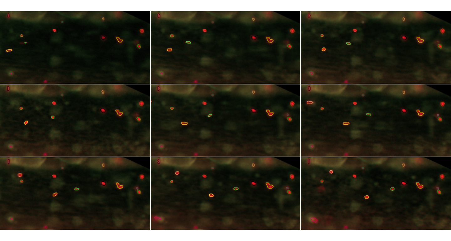
Particles detected in the first 9 frames. These are shown this time in colours corresponding to the identified trajectories, again with their contours defined by the segmentation procedure.
To allow for a thorough evaluation of the single trajectories,
export.Frames is a valid helper, as it creates single
images corresponding to each frame in the Frames object. We
first extract for example trajectory 11 (Fig.@ref(fig:traj11)) with the
following command:
traj11 <- add.contours(raw.frames=MesenteriumSubset,
                       binary.frames=preprocessedPlatelets,
                       trajectoryset=trajPlatelets,
                       mode="trajectories",
                       trajIDs=11)
traj11
## Frames
## colorMode : Color
## storage.mode : double
## dim : 271 131 3 20
## frames.total : 60
## frames.render: 20
##
## imageData(object)[1:5,1:6,1,1]
## [,1] [,2] [,3] [,4] [,5] [,6]
## [1,] 0.1647059 0.2117647 0.1882353 0.1803922 0.1607843 0.1333333
## [2,] 0.2352941 0.1882353 0.1803922 0.1568627 0.1411765 0.1372549
## [3,] 0.2352941 0.2000000 0.1764706 0.1490196 0.1333333 0.1333333
## [4,] 0.2352941 0.2117647 0.1764706 0.1529412 0.1411765 0.1411765
## [5,] 0.2313725 0.2078431 0.1725490 0.1411765 0.1294118 0.1411765
##
## Channel(s): all
inspect.Frames(traj11, nframes=9, display.method="raster")
First 9 frames for trajectory with ID 11. This is supplied to the
trajIds argument of add.contours
The data for trajectory 11 in the TrajectorySet object
can be printed to the terminal:
trajPlatelets[[11]]## $trajectory
## xCoord yCoord trajLabel frame frameobjectID
## 11_1 186.5385 13.84615 11 1 11
## 11_2 186.5000 14.81250 11 2 12
## 11_3 186.4737 14.63158 11 3 11
## 11_4 186.0455 14.45455 11 4 9
## 11_5 186.5000 14.77778 11 5 11
## 11_6 186.5714 15.19048 11 6 12
## 11_7 186.7143 15.42857 11 7 11
## 11_8 186.4286 15.38095 11 8 12
## 11_9 186.0952 15.09524 11 9 11
## 11_10 186.6500 15.30000 11 10 13
## 11_11 186.5714 15.61905 11 11 14
## 11_12 186.7368 15.52632 11 12 12
## 11_13 186.8947 16.05263 11 13 12
## 11_14 186.5000 15.50000 11 14 15
## 11_15 186.8182 15.72727 11 15 13
## 11_16 186.9048 15.95238 11 16 11
## 11_17 186.8636 16.09091 11 17 12
## 11_18 187.0000 16.13636 11 18 11
## 11_19 186.6818 16.13636 11 19 15
## 11_20 186.5789 15.89474 11 20 16
##
## $npoints
## [1] 20
##
## $nframes
## [1] 20
##
## $ngaps
## [1] 0
##
## $keep
## [1] NA
##
## $ID
## [1] 11After that, it can also be exported with the following command (the
dir parameter must be changed accordingly):
export.Frames(traj11, dir=tempdir(), nameStub="vignetteTest_traj11",
              createGif=TRUE, removeAfterCreatingGif=FALSE)
export.Frames offers multiple ways to export - animated
gif (if ImageMagick is available and installed on the
system) or multiple jpeg/png images.
Of course the user might want to singularly evaluate each trajectory that was identified, and this can be done by looping over the trajectory IDs.
evaluatedTrajectories <- trajPlatelets

for(i in 1:length(trajPlatelets))
{
  paintedTraj <- add.contours(raw.frames=MesenteriumSubset,
                              binary.frames=preprocessedPlatelets,
                              trajectoryset=trajPlatelets,
                              mode="trajectories",
                              col="yellow",
                              trajIDs=i)
  export.Frames(paintedTraj,
                nameStub=paste0("vignetteTest_evaluation_traj_oneByOne_",i),
                createGif=TRUE, removeAfterCreatingGif=TRUE)
  ### uncomment the code below to perform the interactive evaluation of the single trajectories

  #   cat("Should I keep this trajectory? --- 0: NO, 1:YES --- no other values allowed")
  #   userInput <- readLines(n=1L)
  #   ## if neither 0 nor 1, do not update
  #   ## otherwise, this becomes the value for the field keep in the new TrajectoryList
  #   evaluatedTrajectories@.Data[[i]]$keep <- as.logical(as.numeric(userInput))
}
Always using trajectory 11 as example, we would set
evaluatedTrajectories[[11]]$keep to TRUE,
since the trajectory was correctly identified, as we just checked.
Once all trajectories have been selected, we can proceed to calculate
(a set of) kinematic parameters, for a single or all trajectories in a
TrajectorySet object. The function kinematics
returns the desired output, respectively a
KinematicsFeatures object, a
KinematicsFeaturesSet, a single value or a vector (or list,
if not coercible to vector) of these single values (one parameter for
each trajectory).
allKinematicFeats.allPlatelets <- kinematics(trajPlatelets,
                                             trajectoryIDs=NULL, # will select all trajectory IDs
                                             acquisitionFrequency=30, # value in milliseconds
                                             scala=50, # 1 pixel is equivalent to ... micrometer
                                             feature=NULL) # all kinematic features available
## Warning in extractKinematics.traj(trajectoryset, i, acquisitionFrequency =
## acquisitionFrequency, : The trajectory with ID 17 had 3 or less points, no
## features were computed.## Warning in extractKinematics.traj(trajectoryset, i, acquisitionFrequency =
## acquisitionFrequency, : The trajectory with ID 18 had 3 or less points, no
## features were computed.## Warning in extractKinematics.traj(trajectoryset, i, acquisitionFrequency =
## acquisitionFrequency, : The trajectory with ID 20 had 3 or less points, no
## features were computed.As it is reported from the output, the function raises a warning for trajectories which have 3 or less points, as they might be spurious detections. In such cases, no kinematic features are computed.
allKinematicFeats.allPlatelets## An object of the KinematicsFeaturesSet class.
##
## KinematicsFeaturesSet composed of 20 KinematicsFeatures objects
##
## Available features (shown for the first trajectory):
## [1] "delta.x" "delta.t"
## [3] "delta.v" "totalTime"
## [5] "totalDistance" "distStartToEnd"
## [7] "curvilinearVelocity" "straightLineVelocity"
## [9] "linearityForwardProgression" "trajMSD"
## [11] "velocityAutoCorr" "instAngle"
## [13] "directChange" "dirAutoCorr"
## [15] "paramsNotComputed"
##
## Curvilinear Velocity: 0.009970094
## Total Distance: 5.682953
## Total Time: 570
##
## Average values (calculated on 3 trajectories where parameters were computed)
## Average Curvilinear Velocity: 0.1278174
## Average Total Distance: 56.08449
## Average Total Time: 518.8235A summary for the returned object (in this case a
KinematicsFeaturesSet) shows some of the computed
parameters. By default, information about the first trajectory is
reported in brief, and the same parameters are evaluated on average
across the selected trajectories. The true values can be accessed in
this case for each trajectory by the subset operator for lists
([[]]), followed by the name of the kinematic feature
(e.g., $totalDistance).
A list of all available parameters is printed with an error message if the user specifies an incorrect name, such as here:
allKinematicFeats.allPlatelets <- kinematics(trajPlatelets, feature="?")## Available features to compute are listed here below.
## Please select one among delta.x, delta.t, delta.v, totalTime,
## totalDistance, distStartToEnd, curvilinearVelocity,
## straightLineVelocity, linearityForwardProgression, trajMSD,
## velocityAutoCorr, instAngle, directChange or dirAutoCorrWhen asking for a single parameter, the value returned is structured in a vector, such that it is straightforward to proceed with further analysis, e.g. by plotting the distribution of the curvilinear velocities (Fig.@ref(fig:allVelos)).
allVelocities <- kinematics(trajPlatelets, feature="curvilinearVelocity")

hist(allVelocities, breaks=10, probability=TRUE, col="cadetblue",
     xlab="Curvilinear Velocities Distribution",
     main="Trajectory Analysis: Curvilinear Velocities")
lines(density(allVelocities, na.rm=TRUE), col="steelblue", lwd=2)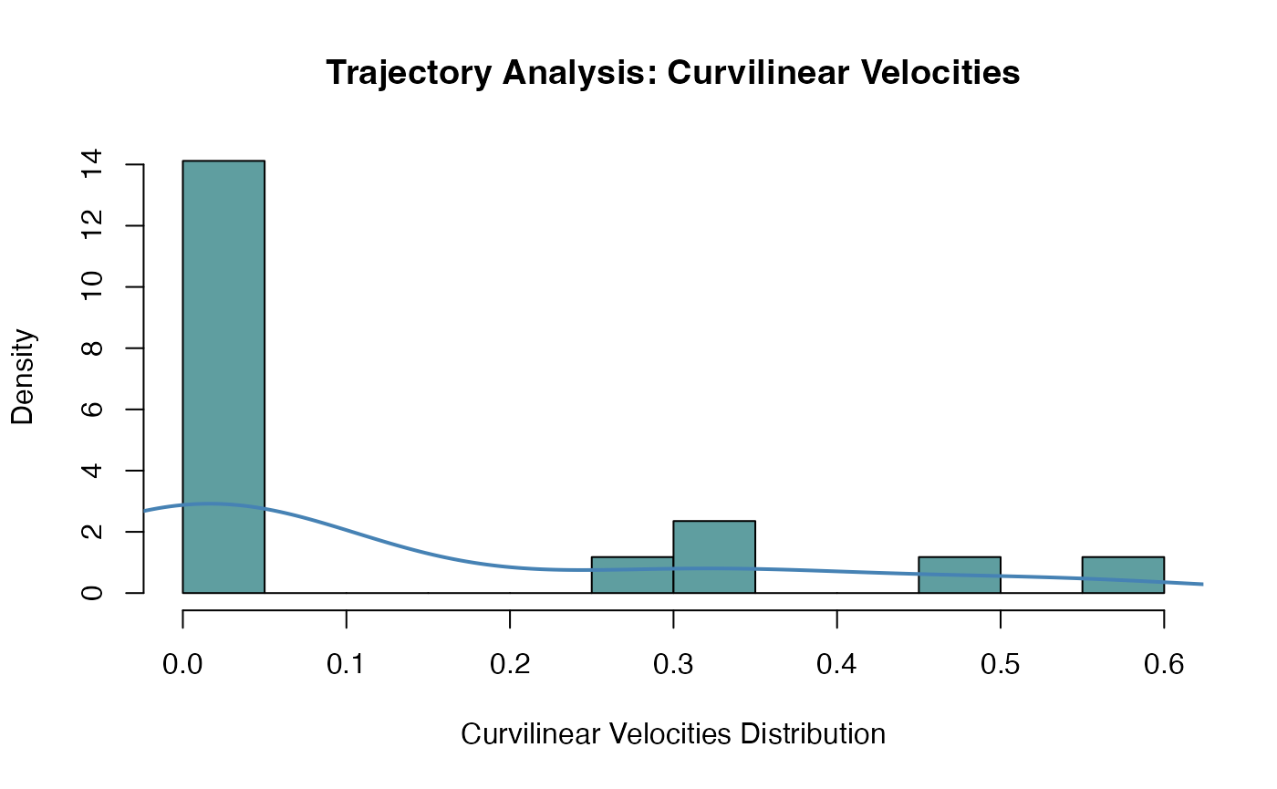
Histogram of the curvilinear velocities for all trajectories identified in the MesenteriumSubset dataset
For this code chunk, we are suppressing the warning messages, as they would be exactly the same as in the former where all features were computed for each trajectory.
Interactive tools for a user-friendly workflow solution
To enhance the Frames objects and deliver an immediate
feedback to the user, the function snap leverages on both
the raw and binary Frames, as well as on the corresponding
ParticleSet and TrajectorySet objects. It
integrates the information available in all the mentioned objects, and
it plots a modified instance of the Frames object,
identifying the particles closest to the mouse click, and showing
additional trajectory-related information, such as the trajectory ID and
the instantaneous velocity of the cell. The function can be called as in
the command below:
snap(MesenteriumSubset,preprocessedPlatelets,
     platelets,trajPlatelets,
     frameID = 1,showVelocity = T)
An example output for the snap is shown below in
Fig.@ref(fig:snapExample), where the information (trajectory ID, as well
as the velocity in the selected frame) is shown in yellow to offer a
good contrast with the fluorescent image.
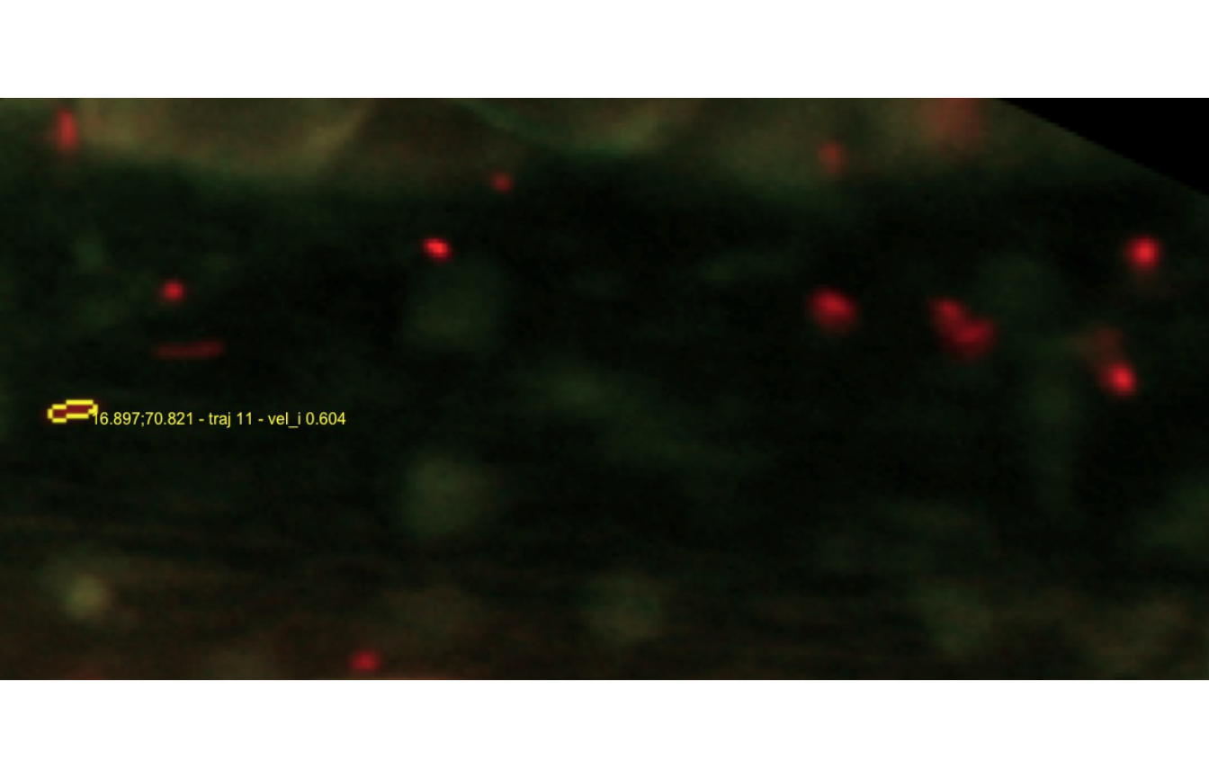
Output generated by the snap function. The user wanted to identify the particle and additionally display the trajectory information (ID, instantaneous velocity) on it.
The shinyFlow Shiny Application
Additionally, since Version 1.0.3, flowcatchR
delivers shinyFlow, a Shiny Web Application ((RStudio, Inc 2013)), which is built on the
backbone of the analysis presented in this vignette, and is portable
across all main operating systems. The user is thus invited to explore
datasets and parameters with immediate reactive feedback, that can
enable better understanding of the effects of single steps and changes
in the workflow.
To launch the Shiny App, use the command below to open an external window either in the browser or in the IDE (such as RStudio):
flowcatchR in Jupyter notebooks
A further integration are a number of Jupyter/IPython notebooks ((Pérez and Granger 2007)), as a way to provide easy reproducibility as well as communication of results, by combining plain text, commands and output in single documents. The R kernel used on the back-end was developed by Thomas Kluyver (https://github.com/takluyver/IRkernel), and instructions for the installation are available at the Github repository website. The notebooks are available in the installation folder of the package flowcatchR, which can be found with the command below.
list.files(system.file("extdata",package = "flowcatchR"),pattern = "*.ipynb")## [1] "template_DetectionOfTransmigrationEvents.ipynb"
## [2] "template_flowcatchR_vignetteSummary.ipynb"The notebooks are provided as template for further steps in the
analysis. The user is invited to set up the IPython notebook framework
as explained on the official website for the project (http://ipython.org/notebook.html). As of February, 3rd
2015, the current way to obtain the Jupyter environment is via the
3.0.dev version, available via Github (https://github.com/ipython/ipython). The notebooks can
be opened and edited by navigating to their location while the IPython
notebook server is running; use the following command in the shell to
launch it:
Alternatively, these documents can be viewed with the
nbviewer tool, available at http://nbviewer.ipython.org/.
flowcatchR in Docker containers
flowcatchR
is now (as of September 2015) available also in Docker images that are
the components of the dockerflow proposal (https://github.com/federicomarini/dockerflow). This
includes:
-
flowstudio- https://github.com/federicomarini/flowstudio, a command-line/IDE interface to RStudio where flowcatchR and its dependencies are preinstalled -
flowshiny- https://github.com/federicomarini/flowshiny a Shiny Server running theshinyFlowweb application -
flowjupy- https://github.com/federicomarini/flowjupy, a Jupyter Notebook interface
These three images can be run simultaneously, provided the system
where the containers are running supports the
docker-compose tool. For more information on how to install
the single components, please refer to their repositories.
Supplementary information
For more information on the method adapted for tracking cells, see Sbalzarini and Koumotsakos (2005) (Sbalzarini and Koumoutsakos 2005). For additional details regarding the functions of flowcatchR, please consult the documentation or write an email to marinif@uni-mainz.de.
Due to space limitations, the complete dataset for the acquired frames used in this vignette is not included as part of the flowcatchR package. If you would like to get access to it, you can write an email to marinif@uni-mainz.de.
Acknowledgements
This package was developed at the Institute of Medical Biostatistics, Epidemiology and Informatics at the University Medical Center, Mainz (Germany), with the financial support provided by the TRP-A15 Translational Research Project grant.
flowcatchR incorporates suggestions and feedback from the wet-lab biology units operating at the Center for Thrombosis and Hemostasis (CTH), in particular Sven Jäckel and Kerstin Jurk. Sven Jäckel also provided us with the sample acquisition which is available in this vignette.
We would like to thank the members of the Biostatistics division for valuable discussions, and additionally Isabella Zwiener for contributing to the first ideas on the project.
Session info
This vignette was generated using the following package versions:
## R Under development (unstable) (2025-11-24 r89053)
## Platform: aarch64-apple-darwin20
## Running under: macOS Sequoia 15.7.2
##
## Matrix products: default
## BLAS:   /System/Library/Frameworks/Accelerate.framework/Versions/A/Frameworks/vecLib.framework/Versions/A/libBLAS.dylib
## LAPACK: /Library/Frameworks/R.framework/Versions/4.6-arm64/Resources/lib/libRlapack.dylib;  LAPACK version 3.12.1
##
## locale:
## [1] en_US.UTF-8/en_US.UTF-8/en_US.UTF-8/C/en_US.UTF-8/en_US.UTF-8
##
## time zone: UTC
## tzcode source: internal
##
## attached base packages:
## [1] stats     graphics  grDevices utils     datasets  methods   base
##
## other attached packages:
## [1] flowcatchR_1.45.0 EBImage_4.53.0    BiocStyle_2.39.0
##
## loaded via a namespace (and not attached):
##  [1] gtable_0.3.6        xfun_0.54           bslib_0.9.0
##  [4] ggplot2_4.0.0       htmlwidgets_1.6.4   lattice_0.22-7
##  [7] crosstalk_1.2.2     vctrs_0.6.5         tools_4.6.0
## [10] bitops_1.0-9        generics_0.1.4      parallel_4.6.0
## [13] tibble_3.3.0        pkgconfig_2.0.3     data.table_1.17.8
## [16] RColorBrewer_1.1-3  S7_0.2.0            desc_1.4.3
## [19] lifecycle_1.0.4     compiler_4.6.0      farver_2.1.2
## [22] textshaping_1.0.4   tiff_0.1-12         codetools_0.2-20
## [25] httpuv_1.6.16       htmltools_0.5.8.1   sass_0.4.10
## [28] RCurl_1.98-1.17     yaml_2.3.10         lazyeval_0.2.2
## [31] plotly_4.11.0       later_1.4.4         pkgdown_2.2.0.9000
## [34] pillar_1.11.1       jquerylib_0.1.4     tidyr_1.3.1
## [37] BiocParallel_1.45.0 cachem_1.1.0        abind_1.4-8
## [40] mime_0.13           tidyselect_1.2.1    locfit_1.5-9.12
## [43] digest_0.6.38       dplyr_1.1.4         purrr_1.2.0
## [46] bookdown_0.45       fastmap_1.2.0       grid_4.6.0
## [49] cli_3.6.5           magrittr_2.0.4      scales_1.4.0
## [52] promises_1.5.0      rmarkdown_2.30      httr_1.4.7
## [55] fftwtools_0.9-11    jpeg_0.1-11         otel_0.2.0
## [58] ragg_1.5.0          png_0.1-8           shiny_1.11.1
## [61] evaluate_1.0.5      knitr_1.50          viridisLite_0.4.2
## [64] rlang_1.1.6         Rcpp_1.1.0          xtable_1.8-4
## [67] glue_1.8.0          BiocManager_1.30.26 BiocGenerics_0.57.0
## [70] jsonlite_2.0.0      R6_2.6.1            systemfonts_1.3.1
## [73] fs_1.6.6            colorRamps_2.3.4