Using quantiseqr • quantiseqr

Introduction

This vignette describes how to use the quantiseqr package for streamlining your workflow around the quanTIseq method. quanTIseq is a transcriptomics deconvolution method that uses an RNA-seq-derived signature matrix (called TIL10) for quantifying 10 different immune cell types in bulk tumor or blood transcriptomics data. quanTIseq has been extensively validated using real and simulated RNA-seq data, as well as flow cytometry and immunohistochemistry data.

The TIL10 signature can quantify cell fractions for

B cells
Classically-activated (M1) macrophages
Alternatively-activated (M2) macrophages
Monocytes
Neutrophils
Natural killer (NK) cells
Non-regulatory (helper) CD4+ T cells
Cytotoxic CD8+ T cells
Regulatory CD4+ T (Treg) cells
Myeloid dendritic cells
Other uncharacterized cells.

For detailed information about quanTIseq methodology and its embedded TIL10 signature, please refer to its original publication (Finotello et al. 2019), or consult the documentation for the quanTIseq pipeline (https://icbi.i-med.ac.at/software/quantiseq/doc/).

quantiseqr returns a cell type by sample quantification of these cell types, either as a simple data frame object, or alternatively, when providing an object derived from the SummarizedExperiment class, adds this information in the colData slot, where it can be further accessed.

Getting started

To install this package, start R and enter:

if (!requireNamespace("BiocManager", quietly = TRUE)) {
  install.packages("BiocManager")
}

BiocManager::install("quantiseqr")

Once installed, the package can be loaded and attached to your current workspace as follows:

library("quantiseqr")

In the following chunk, we load a set of additional packages that will be required throughout this vignette.

library("dplyr")
library("ggplot2")
library("tidyr")
library("tibble")
library("GEOquery")
library("reshape2")
library("SummarizedExperiment")

In order to use quantiseqr in your workflow, one fundamental input is required, to be provided to run_quantiseqr() as expression_data. This is an object containing the gene TPM expression values measured in the sample under investigation, and can be provided in different ways:

as a simple gene expression matrix, or a data frame (with HGNC gene symbols as row names and sample identifiers as column names)
as an ExpressionSet object (from the Biobase package), where the HGNC gene symbols are provided in a column of the fData slot
as a SummarizedExperiment object, or any of the derivative classes (e.g. DESeq2’s DESeqDataSet), in which the assay (default: “abundance”) is containing the TPMs as expected

Some use cases for `quantiseqr`

In this section, we illustrate the usage of quantiseqr on a variety of datasets. These differ with respect to their size and samples of origin, and we illustrate how the different parameters of quantiseqr should be set in the different scenarios.

The fundamental input for quantiseqr is a gene expression matrix-like object, with features on the rows, and samples as the columns. quantiseqr can also directly handle SummarizedExperiment objects, as well as ExpressionSet objects, commonly used for microarray data. In case a SummarizedExperiment object is passed, the quantifications of the immune cell composition can be directly returned extending the colData of the provided input.

Use case 1: Metastatic melanoma patients (Racle et al 2017)

quantiseqr ships with an example dataset with samples from four patients with metastatic melanoma published in (Racle et al. 2017).

The dataset quantiseqr::dataset_racle contains:

a gene expression matrix (dataset_racle$expr_mat) generated using bulk RNA-seq;
‘gold standard’ estimates of immune cell fractions quantified with flow cytometry (dataset_racle$ref).

We are going to use the bulk RNA-seq data to run the deconvolution methods and will compare the results to the FACS data in the following steps.

Let’s inspect the expression matrix first:

data("dataset_racle")
dim(dataset_racle$expr_mat)
#> [1] 32467     4
knitr::kable(dataset_racle$expr_mat[1:5, ])

	LAU125	LAU355	LAU1255	LAU1314
A1BG	0.82	0.58	0.81	0.71
A1CF	0.00	0.01	0.00	0.00
A2M	247.15	24.88	2307.94	20.30
A2M-AS1	1.38	0.20	2.60	0.28
A2ML1	0.03	0.00	0.05	0.02

The quantification of the immune cell types with quantiseqr can be done as in the chunk below:

ti_racle <- quantiseqr::run_quantiseq(
  expression_data = dataset_racle$expr_mat,
  signature_matrix = "TIL10",
  is_arraydata = FALSE,
  is_tumordata = TRUE,
  scale_mRNA = TRUE
)
#> 
#> Running quanTIseq deconvolution module
#> Gene expression normalization and re-annotation (arrays: FALSE)
#> Removing 17 noisy genes
#> Removing 15 genes with high expression in tumors
#> Signature genes found in data set: 135/138 (97.83%)
#> Mixture deconvolution (method: lsei)
#> Deconvolution successful!

The call above means that we are passing the expression data as simple matrix (in dataset_racle$expr_mat) and quantifying the tumor immune cell composition using the (default) TIL10 signature. This is a dataset stemming from tumor RNA-seq samples. Therefore is_tumordata is set to TRUE, whereas is_arraydata is set to FALSE (default). With scale_mRNA set to TRUE (default), we are performing the correction of cell-type-specific mRNA content bias.

The output of quantiseqr can be further processed and visualized in a tabular or graphical manner to facilitate the comparisons across samples/conditions.

The estimates returned by quantiseqr can be interpreted as a cell-type fractions that can be compared between and within samples, making it possible to represent them as a stacked bar chart.

quantiplot(ti_racle)

$Stacked barplot of quanTIseq cell fractions computed on the Racle dataset (patients with metastatic melanoma).$

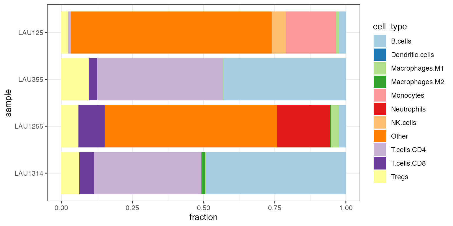
Stacked barplot of quanTIseq cell fractions computed on the Racle dataset (patients with metastatic melanoma).

We observe that

two samples (LAU355, LAU1314) appear to contain a large amount of CD4+ T cells and B cells
the other two samples (LAU1255, LAU125) appear to contain a large amount of “uncharacterized cells”, likely quantifying tumor cell content
one sample (LAU125) appears to contain no CD8+ T cells.

Estimating the amount of “uncharacterized cells” is a novel feature introduced by quanTIseq and EPIC Racle et al. (2017). This estimate often corresponds to the fraction of tumor cells in the sample.

Use case 2: PBMCs from GSE107572 (Finotello et al 2019)

Here we show how to use quantiseqr to deconvolute blood-derived immune-cell mixtures (Finotello et al. 2019), for which also matching flow cytometry data are available.

This is also presented as an example in (Plattner, Finotello, and Rieder 2020), please refer to this later publication for additional details on the processing steps.

The example dataset is available online at the Gene Expression Omnibus (accession number GSE107572), and is provided as preprocessed RNA-seq data from blood-derived immune-cell mixtures from nine healthy donors.
Flow cytometry estimates for the according immune subpopulations are also available.

## While downloading by hand is possible, it is recommended to use GEOquery
# wget -c ftp://ftp.ncbi.nlm.nih.gov/geo/series/GSE107nnn/GSE107572/suppl/GSE107572%5Ftpm%5FPBMC%5FRNAseq%2Etxt%2Egz
# unzip GSE107572_tpm_PBMC_RNAseq.txt.gz
# read.table("GSE107572_tpm_PBMC_RNAseq.txt", header = TRUE)


# downloading the supplemental files on the fly
tpminfo_GSE107572 <- getGEOSuppFiles("GSE107572",
  baseDir = tempdir(),
  filter_regex = "GSE107572_tpm_PBMC_RNAseq"
)
tpm_location <- rownames(tpminfo_GSE107572)[1]
tpm_location
#> [1] "/var/folders/3m/p59k4qdj0f17st0gn2cmj3640000gn/T//RtmpCyTKm0/GSE107572/GSE107572_tpm_PBMC_RNAseq.txt.gz"
tpmdata <- read.table(tpm_location, header = TRUE)

tpm_genesymbols <- tpmdata$GENE
tpmdata <- as.matrix(tpmdata[, -1])
rownames(tpmdata) <- tpm_genesymbols

ti_PBMCs <- quantiseqr::run_quantiseq(
  expression_data = tpmdata,
  signature_matrix = "TIL10",
  is_arraydata = FALSE,
  is_tumordata = FALSE,
  scale_mRNA = TRUE
)
#> 
#> Running quanTIseq deconvolution module
#> Gene expression normalization and re-annotation (arrays: FALSE)
#> Removing 17 noisy genes
#> Signature genes found in data set: 153/153 (100%)
#> Mixture deconvolution (method: lsei)
#> Deconvolution successful!

To obtain an overview on immune cell type compositions, we can print out the results and plot them with the convenient quantiplot wrapper:

# printing out the percentages for the first 4 samples
signif(ti_PBMCs[1:4, 2:12], digits = 3)
#>                        B.cells Macrophages.M1 Macrophages.M2 Monocytes
#> pbmc_1                  0.0929       0.000000         0.0182     0.175
#> pbmc_10                 0.0949       0.000000         0.0113     0.215
#> pbmc_12_merged_1.fastq  0.0643       0.000605         0.0121     0.115
#> pbmc_2_merged_1.fastq   0.0471       0.000000         0.0172     0.152
#>                        Neutrophils NK.cells T.cells.CD4 T.cells.CD8   Tregs
#> pbmc_1                      0.0275  0.02080       0.303       0.225 0.03800
#> pbmc_10                     0.0336  0.00261       0.240       0.196 0.03330
#> pbmc_12_merged_1.fastq      0.0222  0.05580       0.116       0.364 0.00935
#> pbmc_2_merged_1.fastq       0.0546  0.02320       0.238       0.189 0.02830
#>                        Dendritic.cells  Other
#> pbmc_1                          0.0176 0.0827
#> pbmc_10                         0.0326 0.1400
#> pbmc_12_merged_1.fastq          0.0654 0.1750
#> pbmc_2_merged_1.fastq           0.0170 0.2340
# getting a complete visual overview
quantiplot(ti_PBMCs)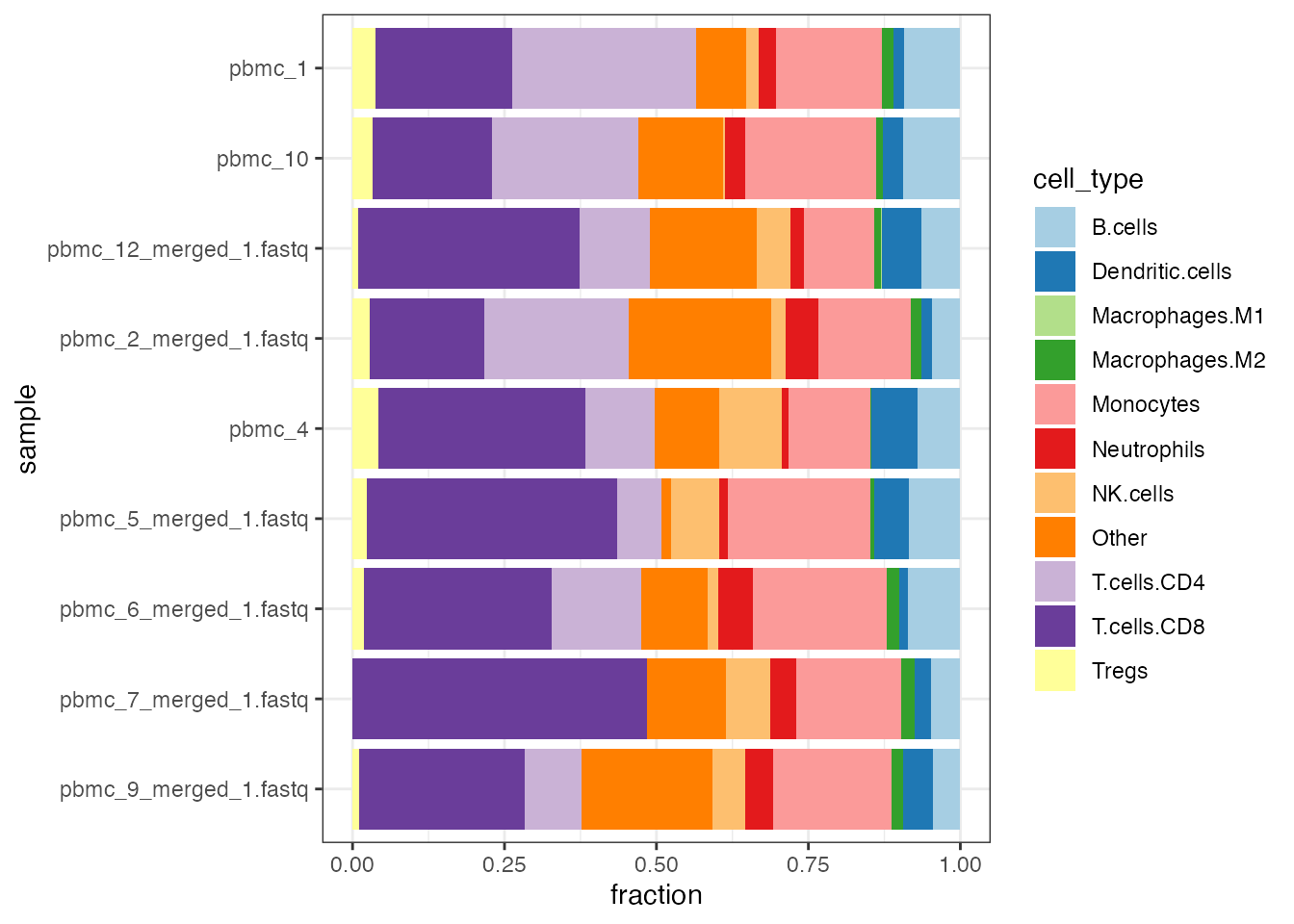

$Stacked barplot of quanTIseq cell fractions computed on the blood derived PBMCs dataset.$

Stacked barplot of quanTIseq cell fractions computed on the blood derived PBMCs dataset.

Notably, for these samples, corresponding quantifications of the true cell fractions done by flow cytometry are also available.
In the chunk that follows, we retrieve that information and generate scatter plots to display how the estimated values from quantiseqr correlate with the ground truth values.
This is adapted by (Plattner, Finotello, and Rieder 2020) to match the output format generated by quantiseqr - and can be used as a template in case other types of matched ground-truth information are available.

We start by retrieving the information from the GSE107572 entry via GEOquery (this will be cached locally after the first execution), and process the information matching it to the quantification of cell fractions we just obtained as ti_PBMCs.

GEOid <- "GSE107572"
gds <- getGEO(GEOid)
#> Found 1 file(s)
#> GSE107572_series_matrix.txt.gz
GEOinfo <- pData(gds[[1]])
FACSdata <- data.frame(
  B.cells = GEOinfo$`b cells:ch1`,
  T.cells.CD4 = GEOinfo$`cd4+ t cells:ch1`,
  T.cells.CD8 = GEOinfo$`cd8+ t cells:ch1`,
  Monocytes = GEOinfo$`monocytes:ch1`,
  Dendritic.cells = GEOinfo$`myeloid dendritic cells:ch1`,
  NK.cells = GEOinfo$`natural killer cells:ch1`,
  Neutrophils = GEOinfo$`neutrophils:ch1`,
  Tregs = GEOinfo$`tregs:ch1`
)
rownames(FACSdata) <- gsub(
  "Blood-derived immune-cell mixture from donor ", "pbmc", GEOinfo$title
)

rownames(ti_PBMCs) <- gsub("_.*$", "", sub("_", "", rownames(ti_PBMCs)))

ccells <- intersect(colnames(ti_PBMCs), colnames(FACSdata))
csbjs <- intersect(rownames(ti_PBMCs), rownames(FACSdata))

ti_PBMCs <- ti_PBMCs[csbjs, ccells]
FACSdata <- FACSdata[csbjs, ccells]

Then we proceed to plot the agreement between the computed cell fractions and the estimated values extracted from flow cytometry experiments.

palette <- c("#451C87", "#B3B300", "#CE0648", "#2363C5", "#AB4CA1", "#0A839B", "#DD8C24", "#ED6D42")

names(palette) <- c("T.cells.CD4", "Dendritic.cells", "Monocytes", "T.cells.CD8", "Tregs", "B.cells", "NK.cells", "Neutrophils")

par(mfrow = c(3, 3))
colall <- c()
for (i in 1:(ncol(ti_PBMCs) + 1)) {
  if (i <= ncol(ti_PBMCs)) {
    x <- as.numeric(as.character(FACSdata[, i]))
    y <- ti_PBMCs[, i]
    ccell <- colnames(ti_PBMCs)[i]
    col <- palette[ccell]
  } else {
    x <- as.numeric(as.vector(as.matrix(FACSdata)))
    y <- as.vector(as.matrix(ti_PBMCs))
    ccell <- "All cells"
    col <- colall
  }
  res.cor <- cor.test(y, x)
  R <- round(res.cor$estimate, digits = 2)
  p <- format.pval(res.cor$p.value, digits = 2)
  RMSE <- round(sqrt(mean((y - x)^2, na.rm = TRUE)), digits = 2)

  regl <- lm(y ~ x)
  ymax <- max(round(max(y), digits = 2) * 1.3, 0.01)
  xmax <- max(round(max(x), digits = 2), 0.01)
  plot(x, y,
    main = gsub("(\\.)", " ", ccell), pch = 19,
    xlab = "Flow cytometry fractions",
    ylab = "quanTIseq cell fractions",
    col = col, cex.main = 1.3, ylim = c(0, ymax), xlim = c(0, xmax), las = 1
  )
  abline(regl)
  abline(a = 0, b = 1, lty = "dashed", col = "lightgrey")
  text(0, ymax * 0.98, cex = 1, paste0("r = ", R, ", p = ", p), pos = 4)
  text(0, ymax * 0.9, cex = 1, paste0("RMSE = ", RMSE), pos = 4)

  colall <- c(colall, rep(col, length(x)))
}

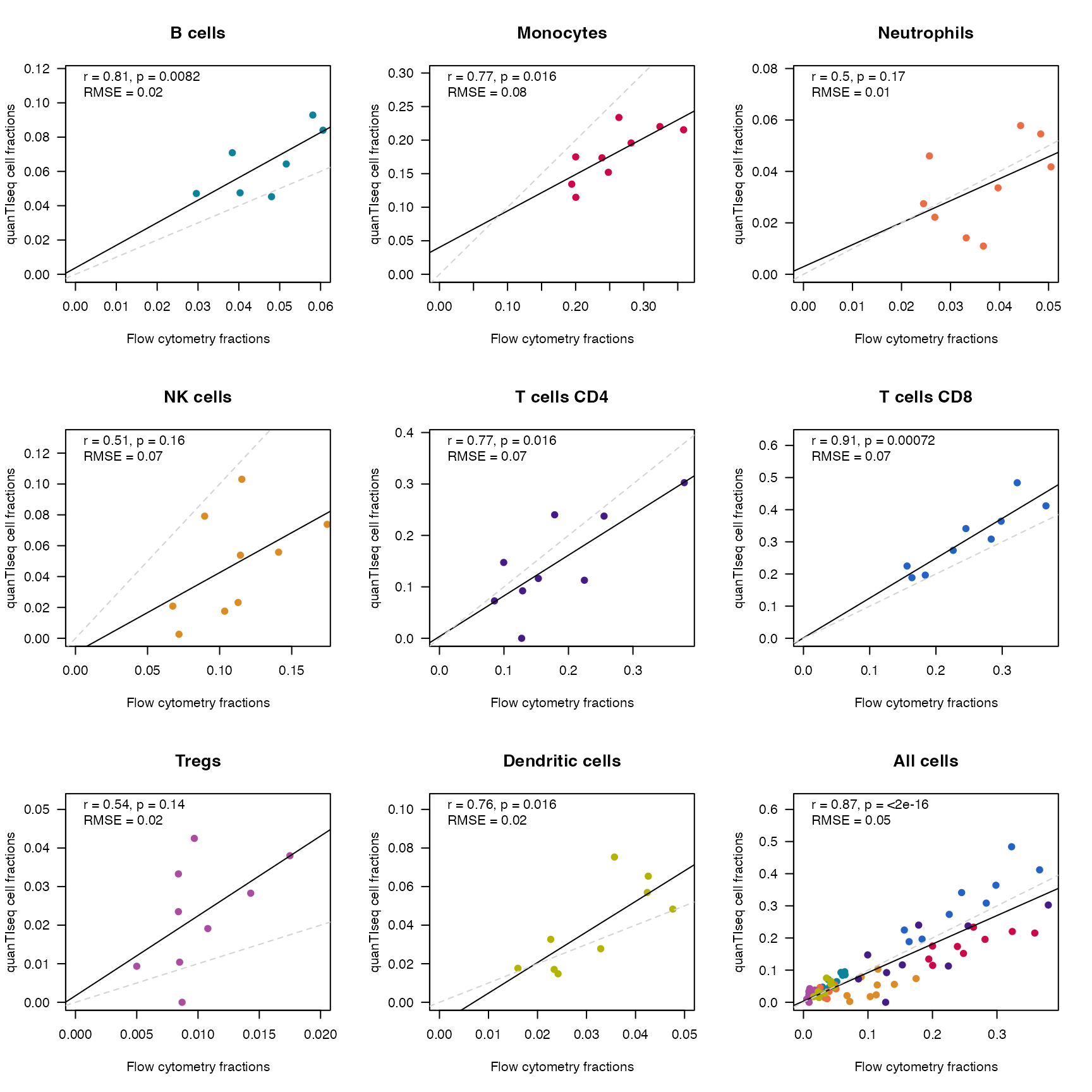
$Scatterplot of quanTIseq cell fractions for the PBMCs dataset, plotted against the fractions estimated from flow cytometry. Each subplot display a specific cell type, and all cells are summarized in the lower right corner. The dashed grey line indicates the diagonal, corresponding to the identity line, while the black solid line is the linear model fit. The text annotation reports the r correlation coefficient, its significance, and the root mean squared error.$

Scatterplot of quanTIseq cell fractions for the PBMCs dataset, plotted against the fractions estimated from flow cytometry. Each subplot display a specific cell type, and all cells are summarized in the lower right corner. The dashed grey line indicates the diagonal, corresponding to the identity line, while the black solid line is the linear model fit. The text annotation reports the r correlation coefficient, its significance, and the root mean squared error.

Use case 3: Expression changes in melanoma patients on vs. pre kinase-inhibitor treatment - GSE75299 (Song et al 2017)

We use here the dataset provided in (Song et al. 2017), where the transcriptomes of cancer cell lines and patients’ tumors were characterized with RNA-seq before and during treatment with kinase inhibitors.

The original dataset is available via GEO at the accession GSE75299, but we will be loading a preprocessed version of it, containing the precomputed TPM expression values, made available via ExperimentHub.
This will enable us to performed a paired analysis on the same observation units (the patients) to appreciate differences in the cell proportions induced by the kinase-inhibitor treatment.

library("ExperimentHub")
#> Loading required package: AnnotationHub
#> Loading required package: BiocFileCache
#> Loading required package: dbplyr
#> 
#> Attaching package: 'dbplyr'
#> The following objects are masked from 'package:dplyr':
#> 
#>     ident, sql
#> 
#> Attaching package: 'AnnotationHub'
#> The following object is masked from 'package:Biobase':
#> 
#>     cache
eh <- ExperimentHub()
quantiseqdata_eh <- query(eh, "quantiseqr")
quantiseqdata_eh
#> ExperimentHub with 1 record
#> # snapshotDate(): 2024-04-29
#> # names(): EH6015
#> # package(): quantiseqr
#> # $dataprovider: GEO
#> # $species: Homo sapiens
#> # $rdataclass: SummarizedExperiment
#> # $rdatadateadded: 2021-04-27
#> # $title: Song2017_MAPKi_treatment
#> # $description: RNA-seq data, quantified as TPM, for tumor samples  pre and ...
#> # $taxonomyid: 9606
#> # $genome: NA
#> # $sourcetype: tar.gz
#> # $sourceurl: https://www.ncbi.nlm.nih.gov/geo/query/acc.cgi?acc=GSE75299
#> # $sourcesize: NA
#> # $tags: c("Annotation", "Classification", "ExperimentHubSoftware",
#> #   "FeatureExtraction", "GeneExpression", "ImmunoOncology",
#> #   "Microarray", "Sequencing", "StatisticalMethod", "Transcription",
#> #   "Transcriptomics", "Visualization") 
#> # retrieve record with 'object[["EH6015"]]'

se_Song2017_MAPKi_treatment <- quantiseqdata_eh[["EH6015"]]
#> see ?quantiseqr and browseVignettes('quantiseqr') for documentation
#> loading from cache

se_Song2017_MAPKi_treatment_tiquant <- quantiseqr::run_quantiseq(
  expression_data = se_Song2017_MAPKi_treatment,
  signature_matrix = "TIL10",
  is_arraydata = FALSE,
  is_tumordata = TRUE,
  scale_mRNA = TRUE
)
#> 
#> Running quanTIseq deconvolution module
#> Gene expression normalization and re-annotation (arrays: FALSE)
#> Removing 17 noisy genes
#> Removing 15 genes with high expression in tumors
#> Signature genes found in data set: 138/138 (100%)
#> Mixture deconvolution (method: lsei)
#> Deconvolution successful!

dim(se_Song2017_MAPKi_treatment_tiquant)
#> [1] 19423    39
# colData(se_Song2017_MAPKi_treatment_tiquant)
colnames(colData(se_Song2017_MAPKi_treatment_tiquant))
#>  [1] "geo_accession"                   "sra_id"                         
#>  [3] "title"                           "status"                         
#>  [5] "submission_date"                 "last_update_date"               
#>  [7] "type"                            "channel_count"                  
#>  [9] "source_name_ch1"                 "organism_ch1"                   
#> [11] "characteristics_ch1"             "characteristics_ch1.1"          
#> [13] "characteristics_ch1.2"           "molecule_ch1"                   
#> [15] "extract_protocol_ch1"            "extract_protocol_ch1.1"         
#> [17] "extract_protocol_ch1.2"          "taxid_ch1"                      
#> [19] "description"                     "description.1"                  
#> [21] "data_processing"                 "data_processing.1"              
#> [23] "data_processing.2"               "data_processing.3"              
#> [25] "platform_id"                     "contact_name"                   
#> [27] "contact_email"                   "contact_department"             
#> [29] "contact_institute"               "contact_address"                
#> [31] "contact_city"                    "contact_state"                  
#> [33] "contact_zip/postal_code"         "contact_country"                
#> [35] "data_row_count"                  "instrument_model"               
#> [37] "library_selection"               "library_source"                 
#> [39] "library_strategy"                "relation"                       
#> [41] "relation.1"                      "relation.2"                     
#> [43] "supplementary_file_1"            "cell line:ch1"                  
#> [45] "mapki treatment:ch1"             "mapki type:ch1"                 
#> [47] "is_patient"                      "quanTIseq_TIL10_B.cells"        
#> [49] "quanTIseq_TIL10_Macrophages.M1"  "quanTIseq_TIL10_Macrophages.M2" 
#> [51] "quanTIseq_TIL10_Monocytes"       "quanTIseq_TIL10_Neutrophils"    
#> [53] "quanTIseq_TIL10_NK.cells"        "quanTIseq_TIL10_T.cells.CD4"    
#> [55] "quanTIseq_TIL10_T.cells.CD8"     "quanTIseq_TIL10_Tregs"          
#> [57] "quanTIseq_TIL10_Dendritic.cells" "quanTIseq_TIL10_Other"

As visible from the output of the last chunk, the cell type composition is stored in the colData slot, if providing a SummarizedExperiment as input.
We first plot the cell fractions by sample, this time with a color palette resembling the one used in (Plattner, Finotello, and Rieder 2020).

# to extract the TIL10-relevant parts:
ti_quant <- quantiseqr::extract_ti_from_se(se_Song2017_MAPKi_treatment_tiquant)
#> Found quantifications for the TIL10 signature...

# to access the full column metadata:
cdata <- colData(se_Song2017_MAPKi_treatment_tiquant)

cellfracs_tidy <- tidyr::pivot_longer(
  as.data.frame(cdata), 
  cols = quanTIseq_TIL10_B.cells:quanTIseq_TIL10_Other)

cellfracs_tidy$name <- factor(gsub("quanTIseq_TIL10_", "", cellfracs_tidy$name),
  levels = c(
    "B.cells", "Macrophages.M1", "Macrophages.M2",
    "Monocytes", "Neutrophils", "NK.cells",
    "T.cells.CD4", "T.cells.CD8", "Tregs",
    "Dendritic.cells", "Other"
  )
)

ggplot(cellfracs_tidy, aes(fill = name, y = value, x = sra_id)) +
  geom_bar(position = "fill", stat = "identity") +
  scale_fill_brewer(palette = "PuOr") +
  xlab("") +
  ylab("Cell Fractions") +
  theme_minimal() +
  theme(axis.text.x = element_text(angle = 45, hjust = 1))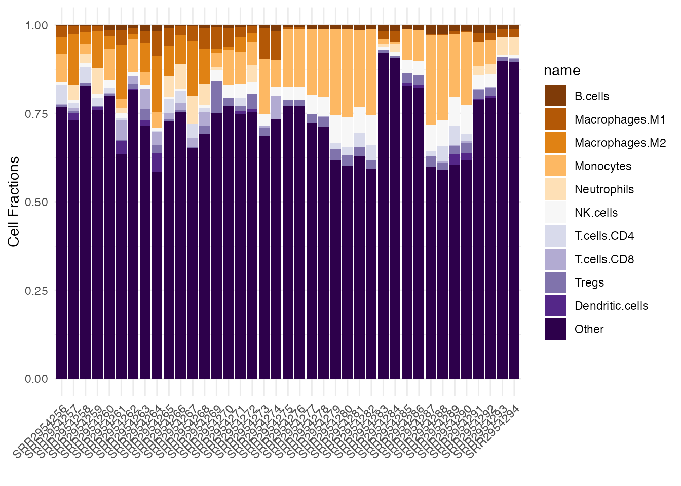

$Stacked barplot of quanTIseq cell fractions computed on the Song et al. dataset, this time using a customized color palette.$

Stacked barplot of quanTIseq cell fractions computed on the Song et al. dataset, this time using a customized color palette.


# we could have also used the compact wrapper
## quantiplot(se_Song2017_MAPKi_treatment_tiquant)

Similarly, we proceed by splitting the data in pre- and post-treatment, first filtering out the cell line samples (keeping the ones where is_patient is TRUE), then manipulating to long format and explicitly building up the plot object.

prepost_data <- cdata[cdata$is_patient, ]

prepost_data_tidy <- tidyr::pivot_longer(
  as.data.frame(prepost_data), 
  cols = quanTIseq_TIL10_B.cells:quanTIseq_TIL10_Dendritic.cells)

prepost_data_tidy$groups <- factor(prepost_data_tidy$mapki.treatment.ch1, levels = c("none", "on-treatment"))

prepost_data_tidy$name <- factor(gsub("quanTIseq_TIL10_", "", prepost_data_tidy$name),
  levels = c(
    "B.cells", "Macrophages.M1", "Macrophages.M2",
    "Monocytes", "Neutrophils", "NK.cells",
    "T.cells.CD4", "T.cells.CD8", "Tregs",
    "Dendritic.cells"
  )
)

ggplot(prepost_data_tidy, aes(name, value, fill = groups)) +
  geom_boxplot() +
  xlab("") +
  ylab("cell fractions") +
  theme_bw() +
  theme(axis.text.x = element_text(angle = 45, hjust = 1))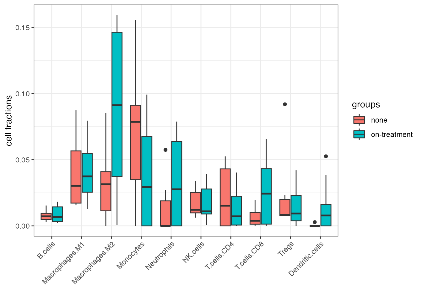

$Boxplot of quanTIseq cell fractions computed on the Song et al. dataset, showing the effect of the MAPKi treatment.$

Boxplot of quanTIseq cell fractions computed on the Song et al. dataset, showing the effect of the MAPKi treatment.

Use case 4: Running on simulated data for validation

We will now display the performance of quantiseqr on a dataset for which the ground truth mRNA fractions are known.
The large simulated dataset represents the RNA-seq expression data from breast tumors with different immune-infiltration scenarios, consisting of a total of 1700 samples, that were generated by mixing RNA-seq reads from purified immune cell types and from a MCF7 breast tumor cell line.

These samples were generated considering different immune relative cell proportions, tumor purity values (0:10:100%), and at different sequencing depths (1, 2, 5, 10, 20, 50, and 100 million read pairs).

Please refer to https://icbi.i-med.ac.at/software/quantiseq/doc/ and to (Finotello et al. 2019) for more details.

This dataset is coupled with a table where the original information on the used true fractions is available, and can be used to benchmark the performance of the deconvolution algorithm.

In this case, we set the scale_mRNA parameter to FALSE because the samples were simulated without modelling any cell-type-specific mRNA bias, so quanTIseq does not have to correct for it. Instead, when analyzing real RNA-seq data, this parameter should always set to TRUE (default) to avoid that some cell types with higher (or lower) total mRNA abundance are systematically under (or over) estimated via deconvolution.

# downloading first the file from https://icbi.i-med.ac.at/software/quantiseq/doc/downloads/quanTIseq_SimRNAseq_mixture.txt

# https://icbi.i-med.ac.at/software/quantiseq/doc/

tpm_1700mixtures <- readr::read_tsv("quanTIseq_SimRNAseq_mixture.txt.gz")
dim(tpm_1700mixtures)

# extracting the gene names, restructuring the matrix by dropping the column
tpm_genesymbols <- tpm_1700mixtures$Gene
tpm_1700mixtures <- as.matrix(tpm_1700mixtures[, -1])
rownames(tpm_1700mixtures) <- tpm_genesymbols

# running quantiseq on that set
# True mRNA fractions were simulated with no total-mRNA bias. Thus, these data should be analyzed specifying the option scale_mRNA set to FALSE
ti_quant_sim1700mixtures <- quantiseqr::run_quantiseq(
  expression_data = tpm_1700mixtures,
  signature_matrix = "TIL10",
  is_arraydata = FALSE,
  is_tumordata = TRUE,
  scale_mRNA = FALSE
)

# save(ti_quant_sim1700mixtures, file = "data/ti_quant_sim1700mixtures.RData")

To avoid the download of a large file, we provide the precomputed object ti_quant_sim1700mixtures in the quantiseqr package - the chunk above is still fully functional once the mixture file has been retrieved.

data(ti_quant_sim1700mixtures)
dim(ti_quant_sim1700mixtures)
#> [1] 1700   12
head(ti_quant_sim1700mixtures)
#>                  Sample     B.cells Macrophages.M1 Macrophages.M2  Monocytes
#> SimData1       SimData1 0.019844435   0.0597686387     0.27196959 0.23806843
#> SimData10     SimData10 0.009382905   0.0249402719     0.08979368 0.09425353
#> SimData100   SimData100 0.033495650   0.0096198517     0.03057850 0.00000000
#> SimData1000 SimData1000 0.042487150   0.0149141815     0.05204647 0.03813509
#> SimData1001 SimData1001 0.029230069   0.0139994722     0.02193008 0.01626132
#> SimData1002 SimData1002 0.013160627   0.0003221679     0.02475316 0.03709523
#>             Neutrophils   NK.cells T.cells.CD4 T.cells.CD8       Tregs
#> SimData1    0.002813382 0.10095469  0.00000000  0.08827795 0.169366189
#> SimData10   0.005454131 0.03922658  0.00000000  0.04532855 0.067272535
#> SimData100  0.016667177 0.04231232  0.00000000  0.04674569 0.010138803
#> SimData1000 0.032586376 0.03811065  0.03650752  0.03029464 0.017042234
#> SimData1001 0.021034018 0.02682053  0.02145636  0.01624266 0.011879932
#> SimData1002 0.007311373 0.01710432  0.00000000  0.01314424 0.008695806
#>             Dendritic.cells     Other
#> SimData1        0.048936698 0.0000000
#> SimData10       0.015406051 0.6089418
#> SimData100      0.023892748 0.7865493
#> SimData1000     0.015217518 0.6826582
#> SimData1001     0.028108596 0.7930370
#> SimData1002     0.001104581 0.8773085
quantiplot(ti_quant_sim1700mixtures[1:100, ])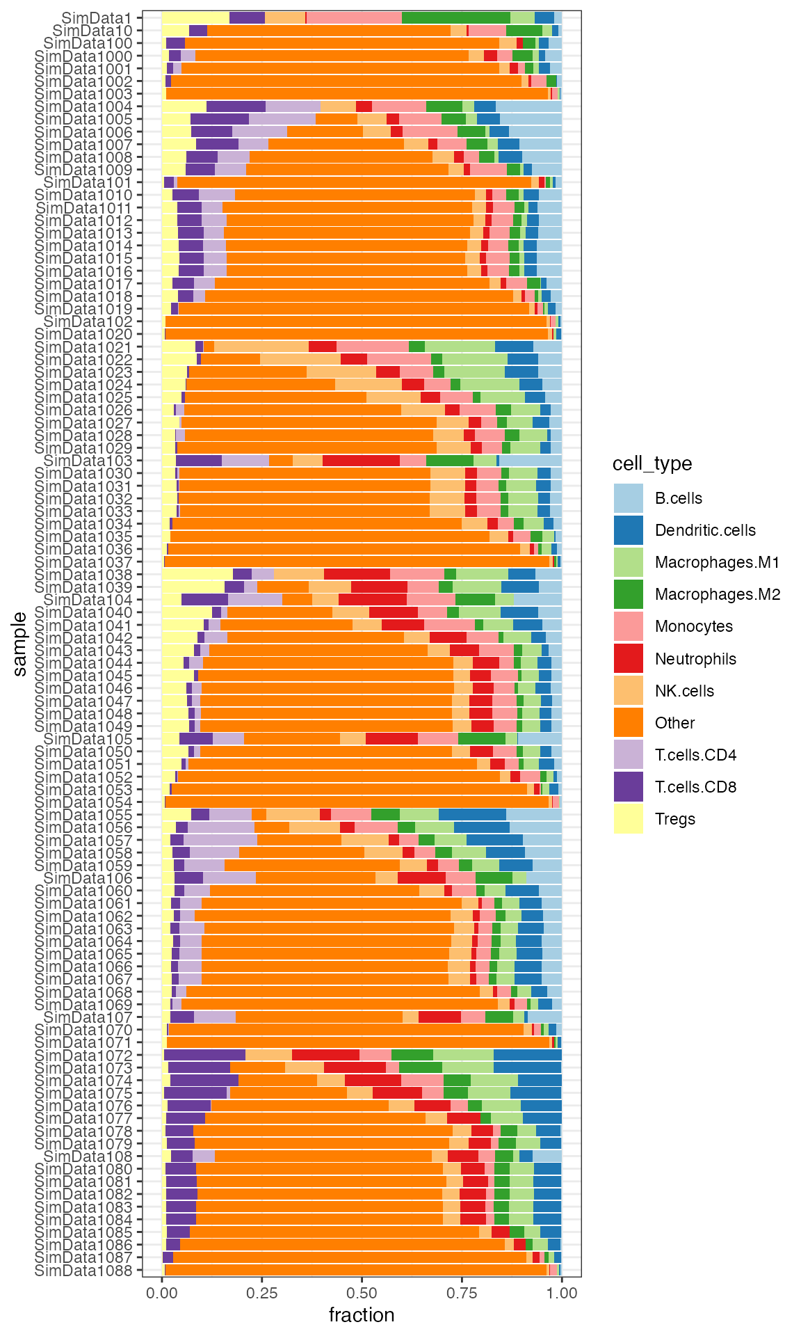

$Stacked barplot of quanTIseq cell fractions computed on the first 100 samples from the simulated dataset.$

Stacked barplot of quanTIseq cell fractions computed on the first 100 samples from the simulated dataset.

We also read in the true proportions, known by design - this is provided as a text file inside quantiseqr.

true_prop_1700mix <- read.table(
  system.file("extdata", "quanTIseq_SimRNAseq_read_fractions.txt.gz", package = "quantiseqr"),
  sep = "\t", header = TRUE
)
head(true_prop_1700mix)
#>           Mix    B.cells Macrophages.M1 Macrophages.M2  Monocytes Neutrophils
#> 1    SimData1 0.01890000    0.067800000     0.22910000 0.22560000 0.007200000
#> 2   SimData10 0.00756000    0.027120000     0.09164000 0.09024000 0.002880000
#> 3  SimData100 0.03178064    0.017140343     0.01076022 0.02004040 0.019540391
#> 4 SimData1000 0.04103877    0.009149726     0.04553863 0.05792826 0.028139156
#> 5 SimData1001 0.02735945    0.006099878     0.03035939 0.03861923 0.018759625
#> 6 SimData1002 0.01367986    0.003049970     0.01517985 0.01930981 0.009379906
#>     NK.cells T.cells.CD4 T.cells.CD8       Tregs Dendritic.cells    Tumor
#> 1 0.09700000  0.00960000 0.108700000 0.203900000     0.032200000 0.000000
#> 2 0.03880000  0.00384000 0.043480000 0.081560000     0.012880000 0.600000
#> 3 0.03480070  0.02140043 0.036440729 0.001720034     0.006360127 0.800016
#> 4 0.03437897  0.03677890 0.029279122 0.012719618     0.005069848 0.699979
#> 5 0.02291954  0.02451951 0.019519610 0.008479830     0.003379932 0.799984
#> 6 0.01145989  0.01225988 0.009759902 0.004239958     0.001689983 0.899991

In the following chunk we perform some preprocessing steps to facilitate the comparison, also in a graphical manner.

# merging the two sets to facilitate the visualization
# colnames(ti_quant_sim1700mixtures) <- paste0("quantiseq_", colnames(ti_quant_sim1700mixtures))
# colnames(true_prop_1700mix) <- paste0("trueprops_", colnames(true_prop_1700mix))

# ti_quant_sim1700mixtures$method <- "quanTIseq"
# true_prop_1700mix$method <- "ground_truth"

colnames(true_prop_1700mix)[1] <- "Sample"
colnames(true_prop_1700mix)[12] <- "Other"

ti_long <- tidyr::pivot_longer(ti_quant_sim1700mixtures,
  cols = B.cells:Other,
  names_to = "cell_type",
  values_to = "value_quantiseq"
)
ti_long$mix_id <- paste(ti_long$Sample, ti_long$cell_type, sep = "_")

tp_long <- pivot_longer(true_prop_1700mix,
  cols = B.cells:Other,
  names_to = "cell_type",
  values_to = "value_trueprop"
)
tp_long$mix_id <- paste(tp_long$Sample, tp_long$cell_type, sep = "_")


ti_tp_merged <- merge(ti_long, tp_long, by = "mix_id")
ti_tp_merged$cell_type.x <- factor(ti_tp_merged$cell_type.x, levels = colnames(true_prop_1700mix)[2:12])

# ti_merged <- rbind(ti_quant_sim1700mixtures,
# true_prop_1700mix)

# ti_merged_long <- pivot_longer(ti_quant_sim1700mixtures, cols = B.cells:Other)

ggplot(
  ti_tp_merged,
  aes(
    x = value_trueprop,
    y = value_quantiseq,
    col = cell_type.x
  )
) +
  geom_point(alpha = 0.5) +
  theme_bw() + 
  labs(
    x = "True fractions",
    y = "quanTIseq cell fractions",
    col = "Cell type"
  )

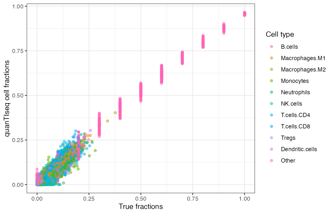
$Scatterplot of quanTIseq cell fractions computed on the simulated dataset, plotted against the true fractions.$

Scatterplot of quanTIseq cell fractions computed on the simulated dataset, plotted against the true fractions.

ggplot(
  ti_tp_merged,
  aes(
    x = value_trueprop,
    y = value_quantiseq,
    col = cell_type.x
  )
) +
  facet_wrap(~cell_type.x, scales = "free") +
  geom_point(alpha = 0.5) +
  geom_abline(slope = 1, col = "lightgrey") + 
  labs(
    x = "True fractions",
    y = "quanTIseq cell fractions",
    col = "Cell type"
  ) + 
  theme_bw()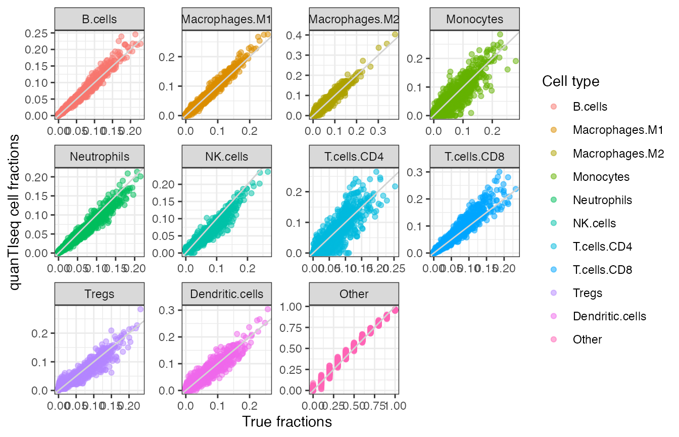

$Scatterplot of quanTIseq cell fractions computed on the simulated dataset, plotted against the true fractions - this time using small multiples for each cell type. The light grey line is the identity line, 'y = x'$

Scatterplot of quanTIseq cell fractions computed on the simulated dataset, plotted against the true fractions - this time using small multiples for each cell type. The light grey line is the identity line, ‘y = x’

This figure aims to replicate with live code the one available as Supplementary Figure 1.

FAQs

Q: Do I have to provide my expression data formatted as TPMs? Why is that so?

A: The expression data is indeed expected to be provided as TPM values. quantiseqr might warn you if you are providing a different format (counts, normalized counts) - this does not mean that it will trigger an error as the computation is still able to proceed.
Still: it is not the recommended way. If using a SummarizedExperiment object coming from Salmon’s quantifications, the tximeta/tximport pipeline will provide an assay named “abundance”, which would be handled internally by the se_to_matrix() function - you can simply call quantiseqr() and provide the SummarizedExperiment object as main parameter.

Q: Can I use quantiseqr with samples from model systems, i.e. not from human?

A: You might exploit orthology-based conversions among gene identifiers to use quantiseqr e.g. in mouse scenarios. Keep in mind, though, that the TIL10 signature has been explicitly designed and validated on human samples.

Q: My expression data is encoding the features in a different identifier than Gene Symbols. Can I use quantiseqr for that?

A: Sure, just make sure to convert the identifiers beforehand - you can use one of the many options available inside Bioconductor for streamlining this step (e.g. the org.Hs.eg.db and the function AnnotationDbi::mapIds()).

Q: I’m interested in other such deconvolution methods. What other options are available?

A: You can check out the works of Sturm, Finotello, and List (2020) to find a collection of methods, provided in the immunedeconv package, and benchmarked in the above mentioned manuscripts.

Q: Can I provide my own signature like the TIL10 and use that in quantiseqr?

A: No, for now it is only possible to use the TIL10 signature matrix.

Session Info

sessionInfo()
#> R version 4.4.0 (2024-04-24)
#> Platform: aarch64-apple-darwin20
#> Running under: macOS Sonoma 14.4.1
#> 
#> Matrix products: default
#> BLAS:   /Library/Frameworks/R.framework/Versions/4.4-arm64/Resources/lib/libRblas.0.dylib 
#> LAPACK: /Library/Frameworks/R.framework/Versions/4.4-arm64/Resources/lib/libRlapack.dylib;  LAPACK version 3.12.0
#> 
#> locale:
#> [1] en_US.UTF-8/en_US.UTF-8/en_US.UTF-8/C/en_US.UTF-8/en_US.UTF-8
#> 
#> time zone: UTC
#> tzcode source: internal
#> 
#> attached base packages:
#> [1] stats4    stats     graphics  grDevices utils     datasets  methods  
#> [8] base     
#> 
#> other attached packages:
#>  [1] ExperimentHub_2.12.0        AnnotationHub_3.12.0       
#>  [3] BiocFileCache_2.12.0        dbplyr_2.5.0               
#>  [5] SummarizedExperiment_1.34.0 GenomicRanges_1.55.4       
#>  [7] GenomeInfoDb_1.40.0         IRanges_2.38.0             
#>  [9] S4Vectors_0.42.0            MatrixGenerics_1.16.0      
#> [11] matrixStats_1.3.0           reshape2_1.4.4             
#> [13] GEOquery_2.72.0             Biobase_2.64.0             
#> [15] BiocGenerics_0.50.0         tibble_3.2.1               
#> [17] tidyr_1.3.1                 ggplot2_3.5.1              
#> [19] dplyr_1.1.4                 quantiseqr_1.13.0          
#> 
#> loaded via a namespace (and not attached):
#>  [1] DBI_1.2.2               rlang_1.1.3             magrittr_2.0.3         
#>  [4] compiler_4.4.0          RSQLite_2.3.6           png_0.1-8              
#>  [7] systemfonts_1.0.6       vctrs_0.6.5             quadprog_1.5-8         
#> [10] stringr_1.5.1           pkgconfig_2.0.3         crayon_1.5.2           
#> [13] fastmap_1.1.1           XVector_0.44.0          labeling_0.4.3         
#> [16] utf8_1.2.4              rmarkdown_2.26.2        tzdb_0.4.0             
#> [19] UCSC.utils_1.0.0        preprocessCore_1.66.0   ragg_1.3.0             
#> [22] purrr_1.0.2             bit_4.0.5               xfun_0.43              
#> [25] zlibbioc_1.50.0         cachem_1.0.8            jsonlite_1.8.8         
#> [28] limSolve_1.5.7.1        blob_1.2.4              highr_0.10             
#> [31] DelayedArray_0.30.0     R6_2.5.1                bslib_0.7.0            
#> [34] stringi_1.8.3           RColorBrewer_1.1-3      limma_3.60.0           
#> [37] jquerylib_0.1.4         Rcpp_1.0.12             knitr_1.46             
#> [40] R.utils_2.12.3          readr_2.1.5             Matrix_1.7-0           
#> [43] tidyselect_1.2.1        abind_1.4-5             yaml_2.3.8             
#> [46] curl_5.2.1              lattice_0.22-6          plyr_1.8.9             
#> [49] KEGGREST_1.44.0         withr_3.0.0             evaluate_0.23          
#> [52] desc_1.4.3              xml2_1.3.6              Biostrings_2.72.0      
#> [55] lpSolve_5.6.20          pillar_1.9.0            BiocManager_1.30.22    
#> [58] filelock_1.0.3          generics_0.1.3          BiocVersion_3.19.1     
#> [61] hms_1.1.3               munsell_0.5.1           scales_1.3.0           
#> [64] BiocStyle_2.32.0        glue_1.7.0              tools_4.4.0            
#> [67] data.table_1.15.4       fs_1.6.4                grid_4.4.0             
#> [70] AnnotationDbi_1.65.2    colorspace_2.1-0        GenomeInfoDbData_1.2.12
#> [73] cli_3.6.2               rappdirs_0.3.3          textshaping_0.3.7      
#> [76] fansi_1.0.6             S4Arrays_1.4.0          gtable_0.3.5           
#> [79] R.methodsS3_1.8.2       sass_0.4.9              digest_0.6.35          
#> [82] SparseArray_1.4.0       farver_2.1.1            memoise_2.0.1          
#> [85] htmltools_0.5.8.1       pkgdown_2.0.9.9000      R.oo_1.26.0            
#> [88] lifecycle_1.0.4         httr_1.4.7              mime_0.12              
#> [91] statmod_1.5.0           bit64_4.0.5             MASS_7.3-60.2

References

Finotello, Francesca, Clemens Mayer, Christina Plattner, Gerhard Laschober, Dietmar Rieder, Hubert Hackl, Anne Krogsdam, et al. 2019. “Molecular and Pharmacological Modulators of the Tumor Immune Contexture Revealed by Deconvolution of RNA-Seq Data.” Genome Medicine 11 (1): 34.

Plattner, Christina, Francesca Finotello, and Dietmar Rieder. 2020. Deconvoluting tumor-infiltrating immune cells from RNA-seq data using quanTIseq. 1st ed. Vol. 636. Elsevier Inc. https://doi.org/10.1016/bs.mie.2019.05.056.

Racle, Julien, Kaat de Jonge, Petra Baumgaertner, Daniel E Speiser, and David Gfeller. 2017. “Simultaneous enumeration of cancer and immune cell types from bulk tumor gene expression data.” eLife 6 (November): e26476. https://doi.org/10.7554/eLife.26476.

Song, Chunying, Marco Piva, Lu Sun, Aayoung Hong, Gatien Moriceau, Xiangju Kong, Hong Zhang, et al. 2017. “Recurrent Tumor Cellintrinsic and Extrinsic Alterations During MAPKi-Induced Melanoma Regression and Early Adaptation.” Cancer Discovery 7 (11): 1248–65. https://doi.org/10.1158/2159-8290.cd-17-0401.

Sturm, Gregor, Francesca Finotello, and Markus List. 2020. “Immunedeconv: An R Package for Unified Access to Computational Methods for Estimating Immune Cell Fractions from Bulk RNA-Sequencing Data.” In, 2120:223–32. Berlin, Boston: DE GRUYTER. https://doi.org/10.1007/978-1-0716-0327-7_16.

Sturm, Gregor, Francesca Finotello, Florent Petitprez, Jitao David Zhang, Jan Baumbach, Wolf H Fridman, Markus List, and Tatsiana Aneichyk. 2019. “Comprehensive Evaluation of Transcriptome-Based Cell-Type Quantification Methods for Immuno-Oncology.” Bioinformatics 35 (14): i436–45.

Federico Marini¹

Francesca Finotello²

2024-05-02

Introduction

Getting started

Some use cases for `quantiseqr`

Use case 1: Metastatic melanoma patients (Racle et al 2017)

Use case 2: PBMCs from GSE107572 (Finotello et al 2019)

Use case 3: Expression changes in melanoma patients on vs. pre kinase-inhibitor treatment - GSE75299 (Song et al 2017)

Use case 4: Running on simulated data for validation

FAQs

Session Info

References

Federico Marini1

Francesca Finotello2

2024-05-02

Introduction

Getting started

Some use cases for quantiseqr

Use case 1: Metastatic melanoma patients (Racle et al 2017)

Use case 2: PBMCs from GSE107572 (Finotello et al 2019)

Use case 3: Expression changes in melanoma patients on vs. pre kinase-inhibitor treatment - GSE75299 (Song et al 2017)

Use case 4: Running on simulated data for validation

FAQs

Session Info

References

Federico Marini¹

Francesca Finotello²

Some use cases for `quantiseqr`