ideal User’s Guide
Federico Marini
Institute of Medical Biostatistics, Epidemiology and Informatics (IMBEI), MainzCenter for Thrombosis and Hemostasis (CTH), Mainzmarinif@uni-mainz.de
Harald Binder
Institute of Medical Biostatistics, Epidemiology and Informatics (IMBEI), Mainz2 May 2025
Source:vignettes/ideal-usersguide.Rmd
ideal-usersguide.RmdAbstract
In the scope of differential expression analysis, we provide the R/Bioconductor package ideal, which serves as a web application to allow simultaneously for interactive and reproducible analysis. ideal guides the user throughout the steps of Differential Expression analysis and produces a wealth of effective visualizations to facilitate data interpretation, in a comprehensive and accessible way for a wide range of scientists.
Package: ideal
Authors: Federico Marini [aut, cre] (ORCID: https://orcid.org/0000-0003-3252-7758)
Version: 2.3.0
Compiled date:
2025-05-02
Last edited: 2019-02-06
License: MIT + file LICENSE

Getting started
ideal is an R package distributed as part of the Bioconductor project. To install the package, start R and enter:
if (!requireNamespace("BiocManager", quietly = TRUE)) {
  install.packages("BiocManager")
}
BiocManager::install("ideal")
The GitHub repository for ideal is https://github.com/federicomarini/ideal. This is the place to file an issue, report a bug, or provide a pull request.
Once ideal is installed, it can be loaded by the following command.
Introduction
ideal is a Bioconductor package containing a Shiny application for analyzing RNA-Seq data in the context of differential expression. This enables an interactive and at the same time analysis, keeping the functionality accessible, and yet providing a comprehensive selection of graphs and tables to mine the dataset at hand.
ideal is an R package which fully leverages the infrastructure of the Bioconductor project in order to deliver an interactive yet reproducible analysis for the detection of differentially expressed genes in RNA-Seq datasets. Graphs, tables, and interactive HTML reports can be readily exported and shared across collaborators. The dynamic user interface displays a broad level of content and information, subdivided by thematic tasks. All in all, it aims to enforce a proper analysis, by reaching out both life scientists and experienced bioinformaticians, and also fosters the communication between the two sides, offering robust statistical methods and high standard of accessible documentation.
It is structured in a similar way to the pcaExplorer, also designed as an interactive companion tool for RNA-seq analysis focused rather on the exploratory data analysis e.g. using principal components analysis as a main tool.
The interactive/reactive design of the app, with a dynamically generated user interface makes it easy and immediate to apply the gold standard methods (in the current implementation, based on DESeq2) in a way that is information-rich and accessible also to the bench biologist, while also providing additional insight also for the experienced data analyst. Reproducibility is supported via state saving and automated report generation.
Citation info
If you use ideal for your analysis, please cite it as here below:
citation("ideal")#> Please cite the articles below for the 'ideal' software itself, or its
#> usage in combined workflows with the 'pcaExplorer' or 'GeneTonic'
#> software packages:
#>
#> Federico Marini, Jan Linke, Harald Binder (2020). ideal: an
#> R/Bioconductor package for Interactive Differential Expression
#> Analysis. BMC Bioinformatics, 21, 565,
#> <doi:10.1186/s12859-020-03819-5> <doi:10.18129/B9.bioc.ideal>.
#>
#> Annekathrin Ludt, Arsenij Ustjanzew, Harald Binder, Konstantin
#> Strauch, Federico Marini (2022). Interactive and Reproducible
#> Workflows for Exploring and Modeling RNA-seq Data with pcaExplorer,
#> ideal, and GeneTonic. Current Protocols, 2 (4), e411,
#> <doi:10.1002/cpz1.411>.
#>
#> To see these entries in BibTeX format, use 'print(<citation>,
#> bibtex=TRUE)', 'toBibtex(.)', or set
#> 'options(citation.bibtex.max=999)'.Using the application
There are different ways to use ideal for interactive differential expression analysis.
Launching ideal locally
First load the library:
and then launch the app with the ideal function. This
takes the following essential parameters as input:
-
dds_obj- aDESeqDataSetobject. If not provided, then acountmatrixand aexpdesignneed to be provided. If none of the above is provided, it is possible to upload the data during the execution of the Shiny App -
res_obj- aDESeqResultsobject. If not provided, it can be computed during the execution of the application -
annotation_obj- adata.frameobject, with row.names as gene identifiers (e.g. ENSEMBL ids) and a column,gene_name, containing e.g. HGNC-based gene symbols. If not provided, it can be constructed during the execution via theorg.eg.XX.dbpackages -
countmatrix- a count matrix, with genes as rows and samples as columns. If not provided, it is possible to upload the data during the execution of the Shiny App -
expdesign-adata.framecontaining the info on the experimental covariates of each sample. If not provided, it is possible to upload the data during the execution of the Shiny App
Different modalities are supported to launch the application:
-
ideal(dds_obj = dds, res_obj = res, annotation_obj = anno), where the objects are precomputed in the current session and provided as parameters -
ideal(dds_obj = dds), as in the command above, but where the result object is assembled at runtime -
ideal(countmatrix = countmatrix, expdesign = expdesign), where instead of passing the definedDESeqDataSetobject, its components are given, namely the count matrix (e.g. generated after a run of featureCounts or HTSeq-count) and a data frame with the experimental covariates. The design formula can be constructed interactively at runtime -
ideal(), where the count matrix and experimental design can simply be uploaded at runtime, where all the derived objects can be extracted and computed live. These files have to be formatted as tabular text files, and a function in the package tries to guess the separator, based on heuristics of occurrencies per line of commonly used characters
You can obtain more information on the formats that are expected and required to work with ideal by pressing the small round button in Step 1 of the Data Setup panel - these are common to the formats used by pcaExplorer. For the sake of completeness, you can see an overview reported in the image below.

The value to specify for the experimental design is best selected
live in Step 2 of the Data Setup panel (see more in Section
@ref(datasetup)) - or if passing directly the dds object in
the call to ideal, is already contained in the
dds itself.
Accessing the public instance of ideal
To use ideal without installing any additional software, you can access the public instance of the Shiny Server made available at the Institute of Medical Biostatistics, Epidemiology and Informatics (IMBEI) in Mainz.
This resource is accessible at this address:
Deploying to a Shiny Server
A deployment-oriented version of the package is available at https://github.com/federicomarini/ideal_serveredition. This repository contains also detailed instruction to setup the running instance of a Shiny Server, where ideal can be run without further installation for the end-users.
Please note that you still need ideal to be installed there once during the setup phase - for this operation, you might require root administrator permissions.
Getting to know the user interface and the functionality
The user interface is dynamically displayed according to the provided and computed objects, with tabs that are actively usable only once the required input is effectively available.
Moreover, for some relevant UI widgets, the user can receive additional information by hovering over with the mouse, with the functionality powered by the shinyBS package.
For the user which is either new with the app UI/functionality, or not extensively familiar with the topic of differential expression, it is possible to obtain a small guided tour of the App by clicking on the respective help buttons, marked in the app like this - please note that this button is clickable but does not start any tour.
These trigger the start of a step-by-step guide and feature introduction, powered by the rintrojs package.
The controls sidebar
Some of the input controls which affect different tabs are located in the sidebar, while others are as well in the individual tabs of the app. By changing one or more of the input parameters, the user can get a fine control on what is computed and displayed.
App settings
- Group/color by - Select the group of samples to stratify the analysis for plotting. Can also assume multiple values.
- Select the gene(s) of interest - ids - Select a subset of genes for deeper analysis. If an annotation object is provided, the user can handily select the genes e.g. based on their HGNC symbol
- False Discovery Rate - Set as default to 0.05, it is the FDR value for the Benjamini-Hochberg procedure for adjusting p-values in the multiple testing comparison scenario
Quick viewer
This displays a list of the underlying objects with which basically all of the analysis can be performed. A green tick icon appears close to each when the respective component is either provided or calculated. For obtaining the best analysis experience in ideal, it is recommended to provide all of them.
The task menu
The task menu, accessible by clicking on the cog icon in the upper right part of the application, provides two functionalities:
-
Exit ideal & savewill close the application and store the content of theinputandvaluesreactive objects in a list of two elements in theideal_envenvironment, respectively calledideal_inputs_YYYYMMDD_HHMMSSandideal_values_YYYYMMDD_HHMMSS -
Save State as .RDatawill similarly storeLiveInputsandr_datain a binary file namedidealState_YYYYMMDD_HHMMSS.Rdata, without closing the application
The main app panels
The ideal app is a one-paged dashboard, structured in different panels, where each of them is focused on a different aspect of the data exploration.
On top of the panels, three valueBox objects serve as
guiding elements for having an overview of the data at hand: how many
genes and samples are in the data, how many entries are in the
annotation object, and how many genes were found to be differentially
expressed in the results. Whenever each of the underlying objects is
available, the background color turns from red to green.
For the main analysis, the available panels are described in the following subsections.
Welcome!
The landing page for the app is also where you might likely be reading this text (otherwise in the package vignette).
Data Setup
The Data Setup panel is where you can upload or inspect the required inputs for running the app. This builds on the primary idea used by pcaExplorer and extends it with the following aspects:
- the panel structure appears dynamically in three consecutive mandatory steps, marked with color from red to yellow to green, with optional steps in light blue.
- the optional step of retrieving the annotation on the fly relieves
the user from the task of composing the
data.framein advance, and is based on the widely adoptedorg.XX.eg.dbBioconductor packages. - when the objects are already passed as parameters, or computed, a brief overview/summary for them is displayed
- to tighten the concert operations between similar tools with different scope (as pcaExplorer and ideal are), the information flow can move from the data exploration to decisions taken at the moment of testing
A diagnostic mean-dispersion plot is also provided in a collapsible
element at the bottom of the panel, shown when the
DESeqDataSet is generated and the DESeq
command from the DESeq2 package has been applied.
Counts Overview
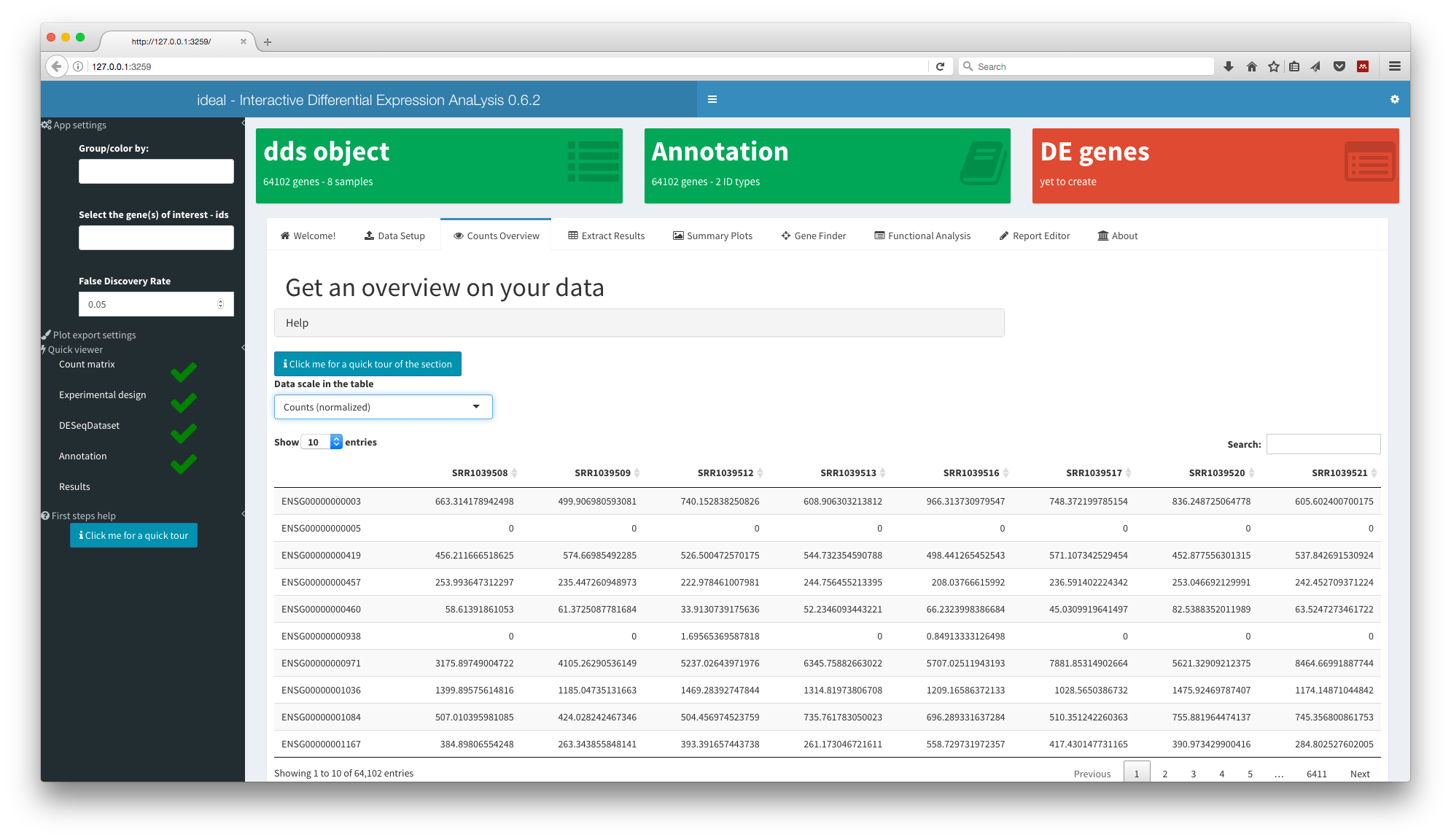
As in pcaExplorer, interactive tables for the raw, normalized, or variance stabilized transformed (preferred over regularized logarithm transformation, because of its speed during the dispersion estimation - especially with larger number of samples) counts are shown in this tab. The user can also generate a sample-to-sample correlation scatter plot with the selected data.
Additionally, ideal has an option to include a filter step at the gene level by removing genes with low absolute or averages low values. After this, it might be possible to have to re-run the analysis in step 3 from the Data Setup panel.
Extract Results
This tab is an interface for generating the summary tables after testing for DE. It is usually based on the Wald test, as implemented in DESeq2, but when the factor of interest is assuming more than two levels, the user can also perform an ANOVA-like test across the groups with the likelihood ratio test. Options for enabling/disabling automated independent filtering, adding the additional column of unshrunken log2 fold change values (instead of the moderated estimates used by default), as well as using the Independent Hypothesis Weighting (IHW) framework, are provided.
The False Discovery Rate (FDR) can be set from the sidebar panel, and a couple of diagnostic plots, such as the histogram of raw p-values and the distribution of log2fc, are shown below the interactive enhanced version of the table - with clickable elements to link to ENSEMBL database and NCBI website.
Summary Plots
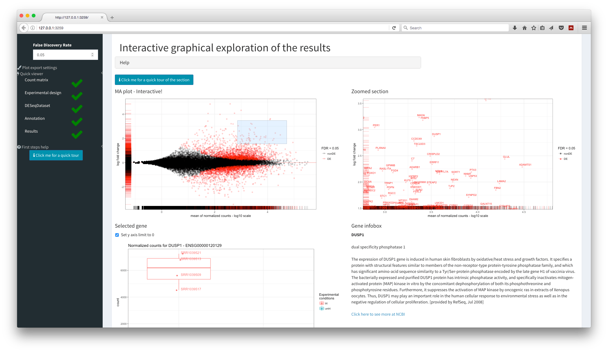
In this tab an interactive MA plot for the contrast selected in the Extract Results tab is displayed. Clicking on a single gene in the zoomed plot (enabled by brushing in the main plot), it is possible to obtain a boxplot for its expression values, flanked by an overview of information accessed live from the Entrez database. Alternatively, a volcano plot of -log10(p-value) versus log fold change can provide a slightly different perspective. The subset of selected genes are also here presented in static and interactive heatmaps, with the underlying data accessible from the collapsible box element.
Gene Finder
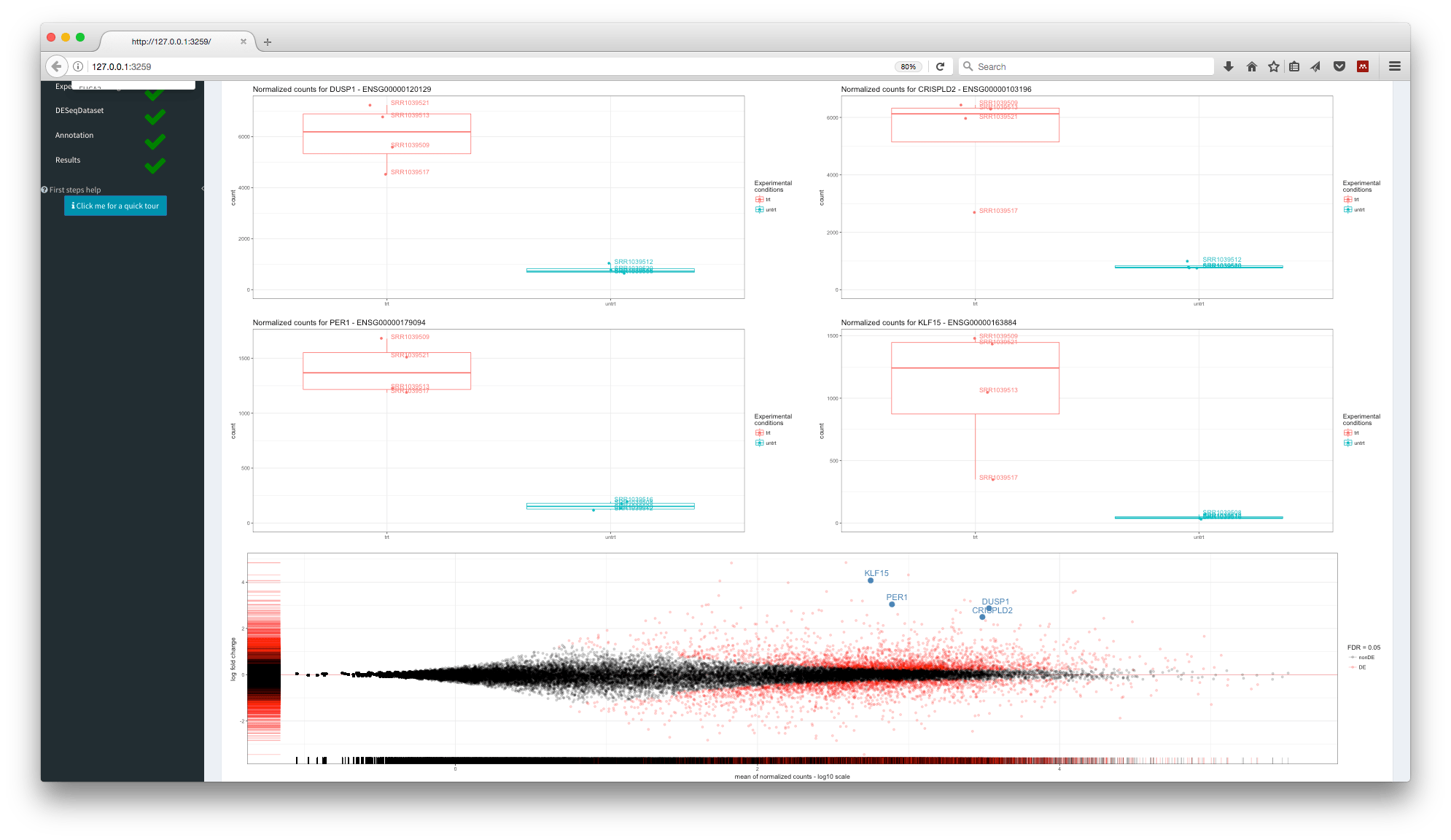
The functionality in the Gene Finder builds upon the one provided by pcaExplorer, and allows to query up to four genes in the same view, which can here be selected from a dropdown input list which supports autocompletion.
A combined summary table (with both normalized counts and results statistics) is located below an MA plot where the selected genes are marked and annotated on the plot. To avoid repeating this manually, the user can also quickly upload a list of genes as text file (one gene identifier per line), such as members of gene families (e.g. all cytokines, all immunoglobulines, …) or defined by common function (e.g. all housekeeping genes, or others based on any annotation).
Functional Analysis
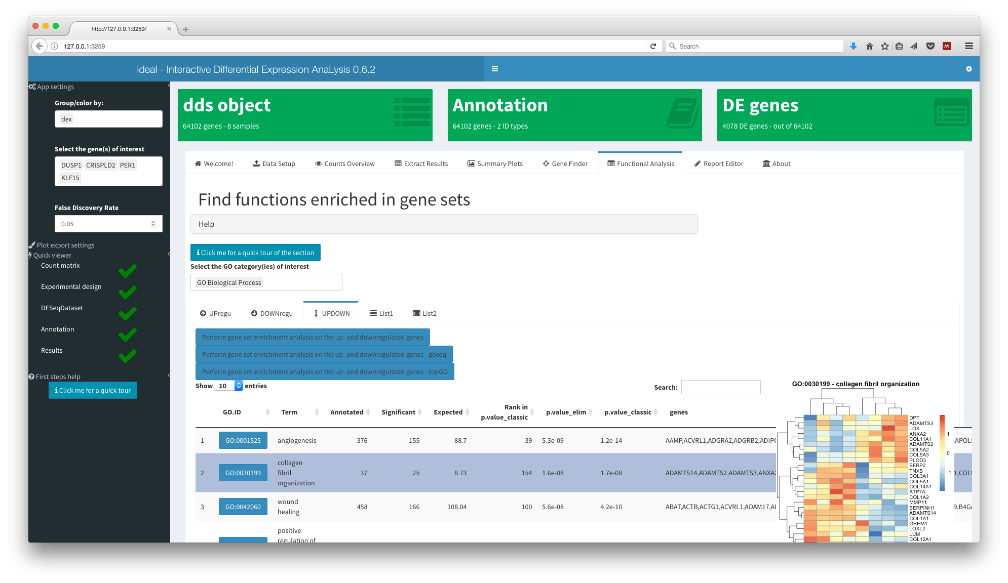
The Functional Analysis tab takes the user from the simple lists of DE genes to insight on the affected biological pathways, with three approaches based on the Gene Ontology (GO) databases. This panel of ideal has a slim interface to the following methods for performing functional analysis:
-
limma::goanafor the quick yet standard implementation -
topGO, particularly valuable for pruning terms which are topologically less meaningful than their specific nodes -
goseq, which accounts for the specific length bias intrinsic in RNA-Seq assays (longer genes have higher chances of being called DE).
ideal allows the user to work simultaneously with more gene lists, two of which can be uploaded in a custom way (e.g. list of gene families, or extracted from other existing publications).
The interaction among these lists can be visually represented in Venn diagrams, as well as with the appealing alternative from the UpSetR package, where all combination of sets are explicitly shown.
Each of the methods for GO enrichment delivers its own interactive
DT-based table, which can then be explored interactively
with the display of a heatmap for all the (DE) genes annotated to a
particular term, picking the normalized transformed values for comparing
robustly the expression values. This is simply triggered by clicking any
of the rows for the results tables. Another useful feature is provided
by the clickable link to the AmiGO database on each of the GO term
identifiers.
Signatures Explorer
The Signatures Explorer tab allows the user to check the behavior of a number of provided gene signatures in the data at hand, displaying this as a heatmap.
This panel is composed by different well panels:
in the Setup Options, you can select and upload a gene signature file, in
gmtformat (e.g. like the ones provided in the MSigDB database, or from WikiPathways), and quickly compute the variance stabilized transformed version of your data, which is more amenable for visualization than raw or normalized countsin the Conversion options tab, you can create an annotation vector, used to bring the ids from your data and the ids the
gmtused for encoding the signature elements. This works based on theorg.XX.eg.dbpackages.the lower well panels control the appearance of the heatmap, also with an option to display all genes annotated in that pathway, or only the ones detected as differentially expressed (for this you need to provide or compute the result object)
Report Editor
The Report Editor tab works in the same way of pcaExplorer, with the scope of providing an interface to full computational reproducibility of the analyses.
General Markdown options and Editor options
are available, and the text editor, based on the shinyAce
package, contains a comprehensive template report, that can be edited to
the best convenience of the user.
The code contained in the template report fetches the latest state of the reactive values in the ongoing session, and its output is a comprehensive HTML file that can be expanded, edited, previewed in the tab itself, downloaded, and shared with a few mouse clicks.
As for pcaExplorer,
the functionality to display the report preview is based on
knit2html, and some elements such as DataTable
objects might not render correctly. To render them correctly, please
install the PhantomJS executable before launching the app. This can be
done by using the webshot
package and calling webshot::install_phantomjs() - HTML
widgets will be rendered automatically as screenshots. Alternatively,
the more recent webshot2
package uses the headless Chrome browser (via the chromote
package, requiring Google Chrome or other Chromium-based browser). Keep
in mind that the fully rendered report (the one you can obtain with the
“Generate & Save” button) is not affected by this, since it uses
rmarkdown::render().
About
The About tab contains the output of sessionInfo, plus
general information on ideal,
including the link to the Github development version. If requested, the
modular structure of the app can be easily expanded, and many new
operations on the same set of input data and derived results can be
embedded in the same framework.
Running ideal on an exemplary data set
We can run ideal for demonstration purpose on published datasets that are available as SummarizedExperiment in an experiment Bioconductor packages.
We will use the airway dataset, which can be installed with this command:
if (!requireNamespace("BiocManager", quietly = TRUE)) {
  install.packages("BiocManager")
}
BiocManager::install("airway")
This package provides a RangedSummarizedExperiment
object of read counts in genes for an RNA-Seq experiment on four human
airway smooth muscle cell lines treated with dexamethasone. More details
such as gene models and count quantifications can be found in the airway
package vignette.
To run ideal on this dataset, the following commands are required. First, prepare the objects to be passed as parameters of ideal.
library("airway")
library("DESeq2")

data("airway", package = "airway")

dds_airway <- DESeqDataSet(airway, design = ~ cell + dex)
dds_airway
#> class: DESeqDataSet
#> dim: 63677 8
#> metadata(2): '' version
#> assays(1): counts
#> rownames(63677): ENSG00000000003 ENSG00000000005 ... ENSG00000273492
#> ENSG00000273493
#> rowData names(10): gene_id gene_name ... seq_coord_system symbol
#> colnames(8): SRR1039508 SRR1039509 ... SRR1039520 SRR1039521
#> colData names(9): SampleName cell ... Sample BioSample
# run deseq on it
dds_airway <- DESeq(dds_airway)
# extract the results
res_airway <- results(dds_airway, contrast = c("dex", "trt", "untrt"), alpha = 0.05)
Then launch the app itself.
ideal(dds_obj = dds_airway)
# or also providing the results object
ideal(dds_obj = dds_airway, res_obj = res_airway)
The annotation for this dataset can be built manually by
exploiting the org.Hs.eg.db
package.
library(org.Hs.eg.db)
genenames_airway <- mapIds(org.Hs.eg.db, keys = rownames(dds_airway), column = "SYMBOL", keytype = "ENSEMBL")
annotation_airway <- data.frame(
  gene_id = rownames(dds_airway),
  gene_name = genenames_airway,
  row.names = rownames(dds_airway),
  stringsAsFactors = FALSE
)
head(annotation_airway)
#> gene_id gene_name
#> ENSG00000000003 ENSG00000000003 TSPAN6
#> ENSG00000000005 ENSG00000000005 TNMD
#> ENSG00000000419 ENSG00000000419 DPM1
#> ENSG00000000457 ENSG00000000457 SCYL3
#> ENSG00000000460 ENSG00000000460 FIRRM
#> ENSG00000000938 ENSG00000000938 FGRor alternatively, can be handily created at runtime in the optional step.
Then again, the app can be launched with:
ideal(
  dds_obj = dds_airway,
  annotation_obj = annotation_airway
)
If desired, alternatives can be used. See the well written annotation workflow available at the Bioconductor site (https://bioconductor.org/help/workflows/annotation/annotation/).
Coming from edgeR/limma-voom
Let’s suppose you performed part of your analysis with edgeR or
limma/voom
and you want to continue inspecting your data interactively using ideal. You
can use the functionality provided by the DEFormats
package to convert the object with:
#> Loading required package: limma#>
#> Attaching package: 'limma'#> The following object is masked from 'package:DESeq2':
#>
#> plotMA#> The following object is masked from 'package:BiocGenerics':
#>
#> plotMA#>
#> Attaching package: 'edgeR'#> The following object is masked from 'package:DEFormats':
#>
#> DGEList
library(limma)
dge_airway <- as.DGEList(dds_airway) # this is your initial object
# your factors for the design:
dex <- colData(dds_airway)$dex
cell <- colData(dds_airway)$cell

redo_dds_airway <- as.DESeqDataSet(dge_airway)
# force the design to ~cell + dex
design(redo_dds_airway) <- ~ cell + group # TODO: this is due to the not 100% re-conversion via DEFormats

### with edgeR
y <- calcNormFactors(dge_airway)
design <- model.matrix(~ cell + dex)
y <- estimateDisp(y, design)
# If you performed quasi-likelihood F-tests
fit <- glmQLFit(y, design)
qlf <- glmQLFTest(fit) # contrast for dexamethasone treatment
topTags(qlf)
#> Coefficient: dexuntrt
#> seqnames
#> ENSG00000109906 11,11,11,11,11,11,11,11,11,11,11,11,11,11,11,11,11,11,11,11,11,11,11,11,11,11,11,11,11,11
#> ENSG00000165995 10,10,10,10,10,10,10,10,10,10,10,10,10,10,10,10,10,10,10,10,10,10,10,10,10,10,10,10,10,10,10,10,10,10
#> ENSG00000250978 5,5,5,5,5,5,5
#> ENSG00000168309 3,3,3,3,3,3,3,3,3,3,3,3,3,3,3,3,3,3
#> ENSG00000152583 4,4,4,4,4,4,4,4,4,4,4,4,4,4,4,4,4,4,4,4,4,4,4,4,4,4,4,4,4,4,4,4,4,4,4,4,4,4,4
#> ENSG00000120129 5,5,5,5
#> ENSG00000189221 X,X,X,X,X,X,X,X,X,X,X,X,X,X,X,X,X,X,X,X,X,X,X,X,X,X,X,X,X
#> ENSG00000146250 6,6,6,6,6
#> ENSG00000171819 1,1,1,1,1,1,1,1
#> ENSG00000157214 7,7,7,7,7,7,7,7,7,7,7,7,7,7,7,7,7,7,7,7,7,7,7,7,7,7,7
#> start
#> ENSG00000109906 113930315,113930447,113930459,113930979,113931229,113932093,113933933,113933933,113933933,113933933,113935134,113992540,114027059,114027059,114051488,114057674,114057674,114057674,114107929,114112889,114112889,114117512,114117920,114117920,114117920,114117920,114121048,114121048,114121048,114121048
#> ENSG00000165995 18429606,18429666,18429676,18429721,18429887,18430109,18439812,18439812,18439812,18470736,18549698,18550190,18629646,18629666,18689742,18690853,18690853,18787284,18787284,18789741,18795400,18803165,18803440,18803909,18807265,18807839,18816517,18823005,18825030,18827109,18828159,18828159,18828159,18828159
#> ENSG00000250978 66759637,66760863,66761082,66762701,66763734,66771243,66771243
#> ENSG00000168309 58549844,58551188,58551188,58551579,58552935,58552946,58555418,58555418,58556053,58563036,58563036,58572585,58574933,58574933,58594601,58612698,58612698,58613143
#> ENSG00000152583 88394487,88394500,88394570,88400582,88401524,88403576,88411425,88411912,88412770,88414734,88414734,88415521,88415521,88415528,88415569,88415592,88415685,88416133,88416133,88416133,88416165,88418283,88420673,88420673,88425974,88449278,88449707,88449707,88450197,88450197,88450197,88450197,88450197,88450197,88450197,88450197,88451697,88452130,88452130
#> ENSG00000120129 172195093,172196578,172197164,172197589
#> ENSG00000189221 43515467,43515548,43515550,43517110,43542761,43542761,43552538,43552538,43571119,43571119,43571119,43571952,43571952,43587420,43587420,43590488,43590488,43590941,43591946,43595474,43599928,43601197,43602951,43603041,43603356,43603356,43603614,43603614,43603614
#> ENSG00000146250 84222194,84222257,84231254,84233141,84233141
#> ENSG00000171819 11249398,11252327,11253637,11253684,11254518,11254583,11254911,11254911
#> ENSG00000157214 89796904,89841000,89841058,89841174,89841187,89841200,89841245,89841590,89843134,89844588,89845805,89845809,89854364,89854364,89854364,89856285,89856285,89856285,89859186,89861651,89861651,89861651,89861651,89866205,89866205,89866205,89867413
#> end
#> ENSG00000109906 113930604,113930604,113930604,113931016,113931306,113932283,113934368,113934466,113935290,113935290,113935290,113992636,114027156,114027156,114051664,114057760,114057760,114060486,114108062,114113059,114113059,114118087,114118018,114118066,114118087,114118087,114121198,114121279,114121374,114121398
#> ENSG00000165995 18429785,18429785,18429785,18429785,18430144,18430144,18439904,18439904,18440198,18471036,18550246,18550246,18629906,18629906,18690029,18690972,18690972,18787406,18787722,18789877,18795476,18803298,18803459,18803970,18807345,18807897,18816626,18823156,18825125,18827294,18828653,18830038,18830056,18830798
#> ENSG00000250978 66759788,66761155,66761155,66762766,66763881,66771305,66771420
#> ENSG00000168309 58552422,58552422,58553091,58552422,58553091,58553091,58555592,58555592,58556150,58563115,58563491,58572840,58574996,58574996,58594984,58613147,58613337,58613337
#> ENSG00000152583 88394955,88394955,88394955,88400730,88401672,88403712,88411545,88412030,88412842,88415750,88415750,88415750,88415750,88415750,88415750,88415750,88415750,88416279,88416279,88416295,88416279,88418391,88420737,88420737,88426075,88449385,88449766,88449771,88450244,88450253,88450393,88450524,88450556,88450609,88450655,88450656,88451783,88452201,88452213
#> ENSG00000120129 172196135,172196797,172197309,172198198
#> ENSG00000189221 43515662,43515662,43515662,43517217,43542855,43542855,43552675,43552675,43571223,43571223,43571223,43572043,43572043,43587561,43587561,43590629,43590637,43591100,43592042,43595527,43599985,43601294,43603152,43603152,43603418,43603418,43603905,43604409,43606068
#> ENSG00000146250 84222413,84222413,84231358,84235419,84235423
#> ENSG00000171819 11250012,11252427,11253831,11253831,11254716,11254716,11255235,11256038
#> ENSG00000157214 89797227,89841359,89841359,89841248,89841359,89841359,89841359,89841650,89843174,89845917,89845917,89845917,89854660,89854888,89854888,89856337,89856347,89856812,89859350,89861798,89861938,89866908,89866945,89866922,89866945,89866992,89867451
#> width
#> ENSG00000109906 290,158,146,38,78,191,436,534,1358,1358,157,97,98,98,177,87,87,2813,134,171,171,576,99,147,168,168,151,232,327,351
#> ENSG00000165995 180,120,110,65,258,36,93,93,387,301,549,57,261,241,288,120,120,123,439,137,77,134,20,62,81,59,110,152,96,186,495,1880,1898,2640
#> ENSG00000250978 152,293,74,66,148,63,178
#> ENSG00000168309 2579,1235,1904,844,157,146,175,175,98,80,456,256,64,64,384,450,640,195
#> ENSG00000152583 469,456,386,149,149,137,121,119,73,1017,1017,230,230,223,182,159,66,147,147,163,115,109,65,65,102,108,60,65,48,57,197,328,360,413,459,460,87,72,84
#> ENSG00000120129 1043,220,146,610
#> ENSG00000189221 196,115,113,108,95,95,138,138,105,105,105,92,92,142,142,142,150,160,97,54,58,98,202,112,63,63,292,796,2455
#> ENSG00000146250 220,157,105,2279,2283
#> ENSG00000171819 615,101,195,148,199,134,325,1128
#> ENSG00000157214 324,360,302,75,173,160,115,61,41,1330,113,109,297,525,525,53,63,528,165,148,288,5258,5295,718,741,788,39
#> strand
#> ENSG00000109906 +,+,+,+,+,+,+,+,+,+,+,+,+,+,+,+,+,+,+,+,+,+,+,+,+,+,+,+,+,+
#> ENSG00000165995 +,+,+,+,+,+,+,+,+,+,+,+,+,+,+,+,+,+,+,+,+,+,+,+,+,+,+,+,+,+,+,+,+,+
#> ENSG00000250978 -,-,-,-,-,-,-
#> ENSG00000168309 -,-,-,-,-,-,-,-,-,-,-,-,-,-,-,-,-,-
#> ENSG00000152583 -,-,-,-,-,-,-,-,-,-,-,-,-,-,-,-,-,-,-,-,-,-,-,-,-,-,-,-,-,-,-,-,-,-,-,-,-,-,-
#> ENSG00000120129 -,-,-,-
#> ENSG00000189221 +,+,+,+,+,+,+,+,+,+,+,+,+,+,+,+,+,+,+,+,+,+,+,+,+,+,+,+,+
#> ENSG00000146250 +,+,+,+,+
#> ENSG00000171819 +,+,+,+,+,+,+,+
#> ENSG00000157214 +,+,+,+,+,+,+,+,+,+,+,+,+,+,+,+,+,+,+,+,+,+,+,+,+,+,+
#> exon_id
#> ENSG00000109906 360958,360959,360960,360961,360962,360963,360964,360965,360967,360966,360968,360969,360971,360970,360972,360974,360973,360975,360976,360977,360978,360979,360980,360981,360982,360983,360984,360985,360986,360987
#> ENSG00000165995 321791,321792,321793,321794,321795,321796,321797,321798,321799,321800,321801,321802,321803,321804,321805,321806,321807,321808,321809,321810,321811,321812,321813,321814,321815,321816,321817,321818,321819,321820,321821,321822,321823,321824
#> ENSG00000250978 199128,199130,199131,199132,199133,199134,199135
#> ENSG00000168309 140728,140729,140730,140731,140732,140733,140734,140735,140736,140737,140738,140739,140741,140740,140742,140743,140744,140745
#> ENSG00000152583 172689,172690,172691,172692,172693,172694,172695,172696,172697,172699,172698,172700,172701,172702,172703,172704,172705,172707,172706,172708,172709,172710,172711,172712,172713,172714,172715,172716,172717,172718,172719,172720,172721,172722,172723,172724,172725,172726,172727
#> ENSG00000120129 207637,207638,207639,207640
#> ENSG00000189221 653982,653983,653984,653985,653986,653987,653989,653988,653990,653991,653992,653993,653994,653995,653996,653997,653998,653999,654000,654001,654002,654003,654004,654005,654006,654007,654008,654009,654010
#> ENSG00000146250 218407,218408,218409,218410,218411
#> ENSG00000171819 2221,2222,2223,2224,2225,2226,2227,2228
#> ENSG00000157214 246728,246730,246731,246732,246733,246734,246735,246736,246737,246738,246739,246740,246741,246743,246742,246744,246745,246746,246747,246748,246749,246750,246751,246752,246753,246754,246755
#> exon_name
#> ENSG00000109906 ENSE00001344383,ENSE00002217296,ENSE00002239785,ENSE00002278969,ENSE00001777728,ENSE00002277816,ENSE00002264739,ENSE00002267450,ENSE00003532715,ENSE00003522546,ENSE00002223922,ENSE00002239280,ENSE00003606532,ENSE00003503866,ENSE00002304588,ENSE00003667676,ENSE00003652618,ENSE00002237247,ENSE00002308595,ENSE00003574983,ENSE00003648066,ENSE00002216844,ENSE00002254046,ENSE00002202712,ENSE00003533854,ENSE00003675344,ENSE00002251269,ENSE00002289800,ENSE00002238115,ENSE00001513888
#> ENSG00000165995 ENSE00001552836,ENSE00001323316,ENSE00001912501,ENSE00001877551,ENSE00001563168,ENSE00001473561,ENSE00003566244,ENSE00003685211,ENSE00001824310,ENSE00001935997,ENSE00001473551,ENSE00001696833,ENSE00001402115,ENSE00001811759,ENSE00001473523,ENSE00003471380,ENSE00003510985,ENSE00001005446,ENSE00001886774,ENSE00001005448,ENSE00001005464,ENSE00001005450,ENSE00001367687,ENSE00001385143,ENSE00001098801,ENSE00001098797,ENSE00001098795,ENSE00001098805,ENSE00001737387,ENSE00001098799,ENSE00001266433,ENSE00001846919,ENSE00001548772,ENSE00001552865
#> ENSG00000250978 ENSE00002085457,ENSE00002055881,ENSE00002051029,ENSE00002080371,ENSE00002028106,ENSE00002048405,ENSE00002074015
#> ENSG00000168309 ENSE00001419495,ENSE00001913711,ENSE00001833888,ENSE00001891124,ENSE00001228325,ENSE00001929708,ENSE00003652265,ENSE00003666445,ENSE00001518622,ENSE00001876866,ENSE00001518624,ENSE00001736715,ENSE00003684332,ENSE00003505632,ENSE00001872799,ENSE00001849960,ENSE00001901828,ENSE00001854286
#> ENSG00000152583 ENSE00001914146,ENSE00001135423,ENSE00002056886,ENSE00001175672,ENSE00001175678,ENSE00001175684,ENSE00001175691,ENSE00001006057,ENSE00001006053,ENSE00003651115,ENSE00003561541,ENSE00003487906,ENSE00003598972,ENSE00001786211,ENSE00002316459,ENSE00002028083,ENSE00001789990,ENSE00003602905,ENSE00003459209,ENSE00002234840,ENSE00001678790,ENSE00002045268,ENSE00003592507,ENSE00003613792,ENSE00001605148,ENSE00002310772,ENSE00002225747,ENSE00002211631,ENSE00002063937,ENSE00002061881,ENSE00002270604,ENSE00002252787,ENSE00002269371,ENSE00001175712,ENSE00001603831,ENSE00001942085,ENSE00002020252,ENSE00002083738,ENSE00002034086
#> ENSG00000120129 ENSE00001876542,ENSE00000769464,ENSE00000769465,ENSE00000812856
#> ENSG00000189221 ENSE00001415055,ENSE00002218265,ENSE00001834008,ENSE00001836223,ENSE00003501661,ENSE00003656032,ENSE00003691177,ENSE00003550793,ENSE00003487993,ENSE00003504764,ENSE00003590154,ENSE00003495252,ENSE00003524833,ENSE00003526715,ENSE00003672501,ENSE00001811266,ENSE00001383783,ENSE00001382812,ENSE00001377890,ENSE00001373498,ENSE00001369566,ENSE00001677475,ENSE00001816354,ENSE00001614970,ENSE00003583432,ENSE00003609031,ENSE00001875207,ENSE00002311052,ENSE00001389556
#> ENSG00000146250 ENSE00002225101,ENSE00001450675,ENSE00002300058,ENSE00002228069,ENSE00001450674
#> ENSG00000171819 ENSE00001471825,ENSE00001168153,ENSE00001168146,ENSE00001948794,ENSE00001168140,ENSE00001823259,ENSE00001841505,ENSE00001471787
#> ENSG00000157214 ENSE00001600835,ENSE00001206871,ENSE00001519027,ENSE00001519061,ENSE00001622820,ENSE00002226827,ENSE00001547971,ENSE00001519060,ENSE00001519048,ENSE00001897780,ENSE00001519046,ENSE00001620946,ENSE00001752071,ENSE00003616543,ENSE00003474395,ENSE00001638606,ENSE00001938466,ENSE00001031278,ENSE00001275182,ENSE00001519045,ENSE00001519014,ENSE00001918233,ENSE00001845894,ENSE00003246458,ENSE00001779097,ENSE00001519026,ENSE00001553338
#> logFC logCPM F PValue FDR
#> ENSG00000109906 -7.133346 4.143740 1525.8323 2.153210e-13 1.371099e-08
#> ENSG00000165995 -3.275414 4.504348 1239.8936 9.820233e-13 3.126615e-08
#> ENSG00000250978 -6.158218 1.348282 398.1877 3.860048e-12 7.978739e-08
#> ENSG00000168309 -4.693470 2.775385 731.1744 5.830619e-12 7.978739e-08
#> ENSG00000152583 -4.547502 5.528678 884.7229 6.265009e-12 7.978739e-08
#> ENSG00000120129 -2.930350 7.308257 757.6713 1.462852e-11 1.552501e-07
#> ENSG00000189221 -3.323171 6.766776 713.3290 2.034469e-11 1.787243e-07
#> ENSG00000146250 2.764572 3.909086 700.7739 2.245386e-11 1.787243e-07
#> ENSG00000171819 -5.700790 3.500283 509.4399 2.818525e-11 1.896165e-07
#> ENSG00000157214 -1.961807 7.129056 644.5267 3.540253e-11 1.896165e-07#> Coefficient: dexuntrt
#> seqnames
#> ENSG00000109906 11,11,11,11,11,11,11,11,11,11,11,11,11,11,11,11,11,11,11,11,11,11,11,11,11,11,11,11,11,11
#> ENSG00000165995 10,10,10,10,10,10,10,10,10,10,10,10,10,10,10,10,10,10,10,10,10,10,10,10,10,10,10,10,10,10,10,10,10,10
#> ENSG00000152583 4,4,4,4,4,4,4,4,4,4,4,4,4,4,4,4,4,4,4,4,4,4,4,4,4,4,4,4,4,4,4,4,4,4,4,4,4,4,4
#> ENSG00000171819 1,1,1,1,1,1,1,1
#> ENSG00000120129 5,5,5,5
#> ENSG00000189221 X,X,X,X,X,X,X,X,X,X,X,X,X,X,X,X,X,X,X,X,X,X,X,X,X,X,X,X,X
#> ENSG00000162692 1,1,1,1,1,1,1,1,1,1,1,1,1,1,1,1
#> ENSG00000168309 3,3,3,3,3,3,3,3,3,3,3,3,3,3,3,3,3,3
#> ENSG00000101347 20,20,20,20,20,20,20,20,20,20,20,20,20,20,20,20,20,20,20,20,20,20,20,20,20,20,20
#> ENSG00000127954 7,7,7,7,7,7,7,7,7,7
#> start
#> ENSG00000109906 113930315,113930447,113930459,113930979,113931229,113932093,113933933,113933933,113933933,113933933,113935134,113992540,114027059,114027059,114051488,114057674,114057674,114057674,114107929,114112889,114112889,114117512,114117920,114117920,114117920,114117920,114121048,114121048,114121048,114121048
#> ENSG00000165995 18429606,18429666,18429676,18429721,18429887,18430109,18439812,18439812,18439812,18470736,18549698,18550190,18629646,18629666,18689742,18690853,18690853,18787284,18787284,18789741,18795400,18803165,18803440,18803909,18807265,18807839,18816517,18823005,18825030,18827109,18828159,18828159,18828159,18828159
#> ENSG00000152583 88394487,88394500,88394570,88400582,88401524,88403576,88411425,88411912,88412770,88414734,88414734,88415521,88415521,88415528,88415569,88415592,88415685,88416133,88416133,88416133,88416165,88418283,88420673,88420673,88425974,88449278,88449707,88449707,88450197,88450197,88450197,88450197,88450197,88450197,88450197,88450197,88451697,88452130,88452130
#> ENSG00000171819 11249398,11252327,11253637,11253684,11254518,11254583,11254911,11254911
#> ENSG00000120129 172195093,172196578,172197164,172197589
#> ENSG00000189221 43515467,43515548,43515550,43517110,43542761,43542761,43552538,43552538,43571119,43571119,43571119,43571952,43571952,43587420,43587420,43590488,43590488,43590941,43591946,43595474,43599928,43601197,43602951,43603041,43603356,43603356,43603614,43603614,43603614
#> ENSG00000162692 101185298,101185311,101185316,101185320,101186032,101186032,101188576,101190180,101194663,101196754,101197974,101200058,101200731,101203679,101203679,101203679
#> ENSG00000168309 58549844,58551188,58551188,58551579,58552935,58552946,58555418,58555418,58556053,58563036,58563036,58572585,58574933,58574933,58594601,58612698,58612698,58613143
#> ENSG00000101347 35518632,35525971,35526225,35526843,35532560,35532560,35533767,35533767,35539621,35540751,35540864,35545125,35545352,35547767,35555585,35555585,35559163,35559163,35563432,35563432,35563744,35569442,35569442,35575141,35575141,35579839,35579839
#> ENSG00000127954 87905744,87907343,87910230,87910798,87911956,87913129,87920231,87936107,87936107,87936107
#> end
#> ENSG00000109906 113930604,113930604,113930604,113931016,113931306,113932283,113934368,113934466,113935290,113935290,113935290,113992636,114027156,114027156,114051664,114057760,114057760,114060486,114108062,114113059,114113059,114118087,114118018,114118066,114118087,114118087,114121198,114121279,114121374,114121398
#> ENSG00000165995 18429785,18429785,18429785,18429785,18430144,18430144,18439904,18439904,18440198,18471036,18550246,18550246,18629906,18629906,18690029,18690972,18690972,18787406,18787722,18789877,18795476,18803298,18803459,18803970,18807345,18807897,18816626,18823156,18825125,18827294,18828653,18830038,18830056,18830798
#> ENSG00000152583 88394955,88394955,88394955,88400730,88401672,88403712,88411545,88412030,88412842,88415750,88415750,88415750,88415750,88415750,88415750,88415750,88415750,88416279,88416279,88416295,88416279,88418391,88420737,88420737,88426075,88449385,88449766,88449771,88450244,88450253,88450393,88450524,88450556,88450609,88450655,88450656,88451783,88452201,88452213
#> ENSG00000171819 11250012,11252427,11253831,11253831,11254716,11254716,11255235,11256038
#> ENSG00000120129 172196135,172196797,172197309,172198198
#> ENSG00000189221 43515662,43515662,43515662,43517217,43542855,43542855,43552675,43552675,43571223,43571223,43571223,43572043,43572043,43587561,43587561,43590629,43590637,43591100,43592042,43595527,43599985,43601294,43603152,43603152,43603418,43603418,43603905,43604409,43606068
#> ENSG00000162692 101185480,101185480,101185480,101185480,101186121,101186307,101188896,101190446,101194938,101197074,101198240,101200324,101204595,101204169,101204594,101204601
#> ENSG00000168309 58552422,58552422,58553091,58552422,58553091,58553091,58555592,58555592,58556150,58563115,58563491,58572840,58574996,58574996,58594984,58613147,58613337,58613337
#> ENSG00000101347 35521469,35526362,35526362,35526947,35532652,35532652,35533797,35533906,35539736,35540955,35540955,35545233,35545452,35547922,35555655,35555655,35559278,35559278,35563592,35563592,35563806,35569514,35569514,35575207,35575207,35580111,35580246
#> ENSG00000127954 87908943,87908943,87910394,87912483,87912483,87913586,87920329,87936195,87936203,87936206
#> width
#> ENSG00000109906 290,158,146,38,78,191,436,534,1358,1358,157,97,98,98,177,87,87,2813,134,171,171,576,99,147,168,168,151,232,327,351
#> ENSG00000165995 180,120,110,65,258,36,93,93,387,301,549,57,261,241,288,120,120,123,439,137,77,134,20,62,81,59,110,152,96,186,495,1880,1898,2640
#> ENSG00000152583 469,456,386,149,149,137,121,119,73,1017,1017,230,230,223,182,159,66,147,147,163,115,109,65,65,102,108,60,65,48,57,197,328,360,413,459,460,87,72,84
#> ENSG00000171819 615,101,195,148,199,134,325,1128
#> ENSG00000120129 1043,220,146,610
#> ENSG00000189221 196,115,113,108,95,95,138,138,105,105,105,92,92,142,142,142,150,160,97,54,58,98,202,112,63,63,292,796,2455
#> ENSG00000162692 183,170,165,161,90,276,321,267,276,321,267,267,3865,491,916,923
#> ENSG00000168309 2579,1235,1904,844,157,146,175,175,98,80,456,256,64,64,384,450,640,195
#> ENSG00000101347 2838,392,138,105,93,93,31,140,116,205,92,109,101,156,71,71,116,116,161,161,63,73,73,67,67,273,408
#> ENSG00000127954 3200,1601,165,1686,528,458,99,89,97,100
#> strand
#> ENSG00000109906 +,+,+,+,+,+,+,+,+,+,+,+,+,+,+,+,+,+,+,+,+,+,+,+,+,+,+,+,+,+
#> ENSG00000165995 +,+,+,+,+,+,+,+,+,+,+,+,+,+,+,+,+,+,+,+,+,+,+,+,+,+,+,+,+,+,+,+,+,+
#> ENSG00000152583 -,-,-,-,-,-,-,-,-,-,-,-,-,-,-,-,-,-,-,-,-,-,-,-,-,-,-,-,-,-,-,-,-,-,-,-,-,-,-
#> ENSG00000171819 +,+,+,+,+,+,+,+
#> ENSG00000120129 -,-,-,-
#> ENSG00000189221 +,+,+,+,+,+,+,+,+,+,+,+,+,+,+,+,+,+,+,+,+,+,+,+,+,+,+,+,+
#> ENSG00000162692 +,+,+,+,+,+,+,+,+,+,+,+,+,+,+,+
#> ENSG00000168309 -,-,-,-,-,-,-,-,-,-,-,-,-,-,-,-,-,-
#> ENSG00000101347 -,-,-,-,-,-,-,-,-,-,-,-,-,-,-,-,-,-,-,-,-,-,-,-,-,-,-
#> ENSG00000127954 -,-,-,-,-,-,-,-,-,-
#> exon_id
#> ENSG00000109906 360958,360959,360960,360961,360962,360963,360964,360965,360967,360966,360968,360969,360971,360970,360972,360974,360973,360975,360976,360977,360978,360979,360980,360981,360982,360983,360984,360985,360986,360987
#> ENSG00000165995 321791,321792,321793,321794,321795,321796,321797,321798,321799,321800,321801,321802,321803,321804,321805,321806,321807,321808,321809,321810,321811,321812,321813,321814,321815,321816,321817,321818,321819,321820,321821,321822,321823,321824
#> ENSG00000152583 172689,172690,172691,172692,172693,172694,172695,172696,172697,172699,172698,172700,172701,172702,172703,172704,172705,172707,172706,172708,172709,172710,172711,172712,172713,172714,172715,172716,172717,172718,172719,172720,172721,172722,172723,172724,172725,172726,172727
#> ENSG00000171819 2221,2222,2223,2224,2225,2226,2227,2228
#> ENSG00000120129 207637,207638,207639,207640
#> ENSG00000189221 653982,653983,653984,653985,653986,653987,653989,653988,653990,653991,653992,653993,653994,653995,653996,653997,653998,653999,654000,654001,654002,654003,654004,654005,654006,654007,654008,654009,654010
#> ENSG00000162692 14792,14793,14794,14795,14796,14797,14798,14799,14800,14801,14802,14803,14804,14805,14806,14807
#> ENSG00000168309 140728,140729,140730,140731,140732,140733,140734,140735,140736,140737,140738,140739,140741,140740,140742,140743,140744,140745
#> ENSG00000101347 626560,626561,626562,626563,626565,626564,626566,626567,626568,626569,626570,626571,626572,626573,626575,626574,626576,626577,626578,626579,626580,626581,626582,626584,626583,626585,626586
#> ENSG00000127954 263537,263538,263539,263540,263541,263542,263543,263544,263545,263546
#> exon_name
#> ENSG00000109906 ENSE00001344383,ENSE00002217296,ENSE00002239785,ENSE00002278969,ENSE00001777728,ENSE00002277816,ENSE00002264739,ENSE00002267450,ENSE00003532715,ENSE00003522546,ENSE00002223922,ENSE00002239280,ENSE00003606532,ENSE00003503866,ENSE00002304588,ENSE00003667676,ENSE00003652618,ENSE00002237247,ENSE00002308595,ENSE00003574983,ENSE00003648066,ENSE00002216844,ENSE00002254046,ENSE00002202712,ENSE00003533854,ENSE00003675344,ENSE00002251269,ENSE00002289800,ENSE00002238115,ENSE00001513888
#> ENSG00000165995 ENSE00001552836,ENSE00001323316,ENSE00001912501,ENSE00001877551,ENSE00001563168,ENSE00001473561,ENSE00003566244,ENSE00003685211,ENSE00001824310,ENSE00001935997,ENSE00001473551,ENSE00001696833,ENSE00001402115,ENSE00001811759,ENSE00001473523,ENSE00003471380,ENSE00003510985,ENSE00001005446,ENSE00001886774,ENSE00001005448,ENSE00001005464,ENSE00001005450,ENSE00001367687,ENSE00001385143,ENSE00001098801,ENSE00001098797,ENSE00001098795,ENSE00001098805,ENSE00001737387,ENSE00001098799,ENSE00001266433,ENSE00001846919,ENSE00001548772,ENSE00001552865
#> ENSG00000152583 ENSE00001914146,ENSE00001135423,ENSE00002056886,ENSE00001175672,ENSE00001175678,ENSE00001175684,ENSE00001175691,ENSE00001006057,ENSE00001006053,ENSE00003651115,ENSE00003561541,ENSE00003487906,ENSE00003598972,ENSE00001786211,ENSE00002316459,ENSE00002028083,ENSE00001789990,ENSE00003602905,ENSE00003459209,ENSE00002234840,ENSE00001678790,ENSE00002045268,ENSE00003592507,ENSE00003613792,ENSE00001605148,ENSE00002310772,ENSE00002225747,ENSE00002211631,ENSE00002063937,ENSE00002061881,ENSE00002270604,ENSE00002252787,ENSE00002269371,ENSE00001175712,ENSE00001603831,ENSE00001942085,ENSE00002020252,ENSE00002083738,ENSE00002034086
#> ENSG00000171819 ENSE00001471825,ENSE00001168153,ENSE00001168146,ENSE00001948794,ENSE00001168140,ENSE00001823259,ENSE00001841505,ENSE00001471787
#> ENSG00000120129 ENSE00001876542,ENSE00000769464,ENSE00000769465,ENSE00000812856
#> ENSG00000189221 ENSE00001415055,ENSE00002218265,ENSE00001834008,ENSE00001836223,ENSE00003501661,ENSE00003656032,ENSE00003691177,ENSE00003550793,ENSE00003487993,ENSE00003504764,ENSE00003590154,ENSE00003495252,ENSE00003524833,ENSE00003526715,ENSE00003672501,ENSE00001811266,ENSE00001383783,ENSE00001382812,ENSE00001377890,ENSE00001373498,ENSE00001369566,ENSE00001677475,ENSE00001816354,ENSE00001614970,ENSE00003583432,ENSE00003609031,ENSE00001875207,ENSE00002311052,ENSE00001389556
#> ENSG00000162692 ENSE00001167786,ENSE00001811760,ENSE00001825682,ENSE00001451872,ENSE00001451878,ENSE00001067757,ENSE00001067755,ENSE00001067758,ENSE00001067756,ENSE00001067753,ENSE00001067759,ENSE00001067751,ENSE00003565397,ENSE00001892498,ENSE00001451871,ENSE00001167778
#> ENSG00000168309 ENSE00001419495,ENSE00001913711,ENSE00001833888,ENSE00001891124,ENSE00001228325,ENSE00001929708,ENSE00003652265,ENSE00003666445,ENSE00001518622,ENSE00001876866,ENSE00001518624,ENSE00001736715,ENSE00003684332,ENSE00003505632,ENSE00001872799,ENSE00001849960,ENSE00001901828,ENSE00001854286
#> ENSG00000101347 ENSE00000800455,ENSE00001930417,ENSE00000661812,ENSE00000661813,ENSE00003692177,ENSE00003551249,ENSE00001842453,ENSE00000661815,ENSE00001622813,ENSE00001604475,ENSE00001711142,ENSE00001793017,ENSE00001667406,ENSE00001752622,ENSE00003598833,ENSE00003555165,ENSE00003535434,ENSE00003608826,ENSE00003546823,ENSE00003559540,ENSE00002218059,ENSE00003462531,ENSE00003673643,ENSE00003619308,ENSE00003541183,ENSE00001957470,ENSE00001898623
#> ENSG00000127954 ENSE00001917465,ENSE00001277946,ENSE00001163797,ENSE00001753614,ENSE00001483677,ENSE00001120706,ENSE00001621319,ENSE00001673636,ENSE00001905312,ENSE00001871078
#> logFC logCPM LR PValue FDR
#> ENSG00000109906 -7.142190 4.143740 1277.6447 8.154169e-280 5.192330e-275
#> ENSG00000165995 -3.274796 4.504348 826.0713 1.158242e-181 3.687670e-177
#> ENSG00000152583 -4.554996 5.528678 693.6567 7.163187e-153 1.520434e-148
#> ENSG00000171819 -5.666372 3.500283 602.1496 5.704778e-133 9.081579e-129
#> ENSG00000120129 -2.932425 7.308257 554.3550 1.421037e-122 1.809747e-118
#> ENSG00000189221 -3.336778 6.766776 544.9495 1.580103e-120 1.676937e-116
#> ENSG00000162692 3.686533 4.599336 530.9701 1.737408e-117 1.580471e-113
#> ENSG00000168309 -4.723461 2.775385 505.4801 6.103995e-112 4.858551e-108
#> ENSG00000101347 -3.751832 9.206504 498.2099 2.330547e-110 1.648914e-106
#> ENSG00000127954 -5.175401 3.652849 491.7830 5.832387e-109 3.713889e-105
# lrt to DESeqResults

tbledger <- lrt$table
colnames(tbledger)[colnames(tbledger) == "PValue"] <- "pvalue"
colnames(tbledger)[colnames(tbledger) == "logFC"] <- "log2FoldChange"
colnames(tbledger)[colnames(tbledger) == "logCPM"] <- "baseMean"
# get from the logcpm to something more the baseMean for better
tbledger$baseMean <- (2^tbledger$baseMean) * mean(dge_airway$samples$lib.size) / 1e6
# use the constructor for DESeqResults
edger_resu <- DESeqResults(DataFrame(tbledger))
edger_resu <- DESeq2:::pvalueAdjustment(edger_resu,
  independentFiltering = TRUE,
  alpha = 0.05, pAdjustMethod = "BH"
)

# cfr with res_airway
# plot(res_airway$pvalue,edger_resu$pvalue)


### with limma-voom
x <- calcNormFactors(dge_airway)
design <- model.matrix(~ 0 + dex + cell)
contr.matrix <- makeContrasts(dextrt - dexuntrt, levels = colnames(design))
v <- voom(x, design)
vfit <- lmFit(v, design)
vfit <- contrasts.fit(vfit, contrasts = contr.matrix)
efit <- eBayes(vfit)

tbllimma <- topTable(efit, number = Inf, sort.by = "none")
colnames(tbllimma)[colnames(tbllimma) == "P.Value"] <- "pvalue"
colnames(tbllimma)[colnames(tbllimma) == "logFC"] <- "log2FoldChange"
colnames(tbllimma)[colnames(tbllimma) == "AveExpr"] <- "baseMean"
colnames(tbllimma)[colnames(tbllimma) == "adj.P.Val"] <- "padj"
# get from the logcpm to something more the baseMean for better
tbllimma$baseMean <- (2^tbllimma$baseMean) * mean(dge_airway$samples$lib.size) / 1e6
# use the constructor for DESeqResults
limma_resu <- DESeqResults(DataFrame(tbllimma))

# cfr with res_airway
# plot(res_airway$pvalue,limma_resu$pvalue)
After preparing the objects, you can launch the app with the following command:
Basically, you need a data.frame
(e.g. myresults_df) with 3 columns to create the
DESeqResults object to be passed to the app, with this
names:
-
baseMeanas an average expression value -
log2FoldChangeas an indicator for the effect size -
pvalueas a measure of significance
Then, you just need to call
DESeqResults(DataFrame(myresults_df)). padj
can be computed either by p.adjust or using
DESeq2:::pvalueAdjustment as in the example above.
Functions exported by the package for standalone usage
The functions exported by the ideal package can be also used in a standalone scenario, provided the required objects are in the working environment. They are listed here for an overview, but please refer to the documentation for additional details. Where possible, for each function a code snippet will be provided for its typical usage.
deseqresult2DEgenes and
deseqresult2tbl
deseqresult2DEgenes and deseqresult2tbl
generate a tidy table with the results of DESeq2, sorted by the values
in the padj column.
From version 1.30.0 onwards, the deseqresult2tbl() and
deseqresult2DEgenes() functions have been deprecated, in
favor of the equivalent mosdef::deresult_to_df() function,
which is more robust and flexible in its usage.
summary(res_airway)#>
#> out of 33469 with nonzero total read count
#> adjusted p-value < 0.05
#> LFC > 0 (up) : 2211, 6.6%
#> LFC < 0 (down) : 1817, 5.4%
#> outliers [1] : 0, 0%
#> low counts [2] : 16687, 50%
#> (mean count < 7)
#> [1] see 'cooksCutoff' argument of ?results
#> [2] see 'independentFiltering' argument of ?results
res_airway#> log2 fold change (MLE): dex trt vs untrt
#> Wald test p-value: dex trt vs untrt
#> DataFrame with 63677 rows and 6 columns
#> baseMean log2FoldChange lfcSE stat pvalue
#> <numeric> <numeric> <numeric> <numeric> <numeric>
#> ENSG00000000003 708.6022 -0.3812540 0.100654 -3.787752 0.000152016
#> ENSG00000000005 0.0000 NA NA NA NA
#> ENSG00000000419 520.2979 0.2068126 0.112219 1.842943 0.065337292
#> ENSG00000000457 237.1630 0.0379204 0.143445 0.264356 0.791505742
#> ENSG00000000460 57.9326 -0.0881682 0.287142 -0.307054 0.758801924
#> ... ... ... ... ... ...
#> ENSG00000273489 0.275899 1.483738 3.51395 0.422243 0.672848
#> ENSG00000273490 0.000000 NA NA NA NA
#> ENSG00000273491 0.000000 NA NA NA NA
#> ENSG00000273492 0.105978 -0.463679 3.52308 -0.131612 0.895291
#> ENSG00000273493 0.106142 -0.521355 3.53139 -0.147634 0.882631
#> padj
#> <numeric>
#> ENSG00000000003 0.00119659
#> ENSG00000000005 NA
#> ENSG00000000419 0.18625623
#> ENSG00000000457 0.90370473
#> ENSG00000000460 0.88616659
#> ... ...
#> ENSG00000273489 NA
#> ENSG00000273490 NA
#> ENSG00000273491 NA
#> ENSG00000273492 NA
#> ENSG00000273493 NA
head(mosdef::deresult_to_df(res_airway))#> id baseMean log2FoldChange lfcSE stat
#> ENSG00000152583 ENSG00000152583 997.4398 4.574919 0.1840561 24.85611
#> ENSG00000165995 ENSG00000165995 495.0929 3.291062 0.1331737 24.71255
#> ENSG00000120129 ENSG00000120129 3409.0294 2.947810 0.1214377 24.27426
#> ENSG00000101347 ENSG00000101347 12703.3871 3.766995 0.1554380 24.23472
#> ENSG00000189221 ENSG00000189221 2341.7673 3.353580 0.1417823 23.65301
#> ENSG00000211445 ENSG00000211445 12285.6151 3.730403 0.1658306 22.49526
#> pvalue padj
#> ENSG00000152583 2.220933e-136 3.727170e-132
#> ENSG00000165995 7.839410e-135 6.578049e-131
#> ENSG00000120129 3.666925e-130 2.051278e-126
#> ENSG00000101347 9.583815e-130 4.020890e-126
#> ENSG00000189221 1.098955e-123 3.688532e-120
#> ENSG00000211445 4.618318e-112 1.291744e-108In particular, deseqresult2DEgenes only includes genes
detected as DE - this is also covered by
mosdef::deresult_to_df() in the newer versions.
head(mosdef::deresult_to_df(res_airway, FDR = 0.05))#> id baseMean log2FoldChange lfcSE stat
#> ENSG00000152583 ENSG00000152583 997.4398 4.574919 0.1840561 24.85611
#> ENSG00000165995 ENSG00000165995 495.0929 3.291062 0.1331737 24.71255
#> ENSG00000120129 ENSG00000120129 3409.0294 2.947810 0.1214377 24.27426
#> ENSG00000101347 ENSG00000101347 12703.3871 3.766995 0.1554380 24.23472
#> ENSG00000189221 ENSG00000189221 2341.7673 3.353580 0.1417823 23.65301
#> ENSG00000211445 ENSG00000211445 12285.6151 3.730403 0.1658306 22.49526
#> pvalue padj
#> ENSG00000152583 2.220933e-136 3.727170e-132
#> ENSG00000165995 7.839410e-135 6.578049e-131
#> ENSG00000120129 3.666925e-130 2.051278e-126
#> ENSG00000101347 9.583815e-130 4.020890e-126
#> ENSG00000189221 1.098955e-123 3.688532e-120
#> ENSG00000211445 4.618318e-112 1.291744e-108
# the output in the first lines is the same, but
dim(res_airway)
#> [1] 63677 6
dim(mosdef::deresult_to_df(res_airway))#> [1] 63677 7This tables can be enhanced with clickable links to the ENSEMBL and NCBI gene databases by the following commands:
myde <- mosdef::deresult_to_df(res_airway, FDR = 0.05)
myde$symbol <- mapIds(org.Hs.eg.db, keys = as.character(myde$id), column = "SYMBOL", keytype = "ENSEMBL")
#> 'select()' returned 1:many mapping between keys and columns
myde_enhanced <- myde
myde_enhanced$id <- mosdef::create_link_ENSEMBL(myde_enhanced$id, species = "Homo_sapiens")
myde_enhanced$symbol <- mosdef::create_link_NCBI(myde_enhanced$symbol)

DT::datatable(myde_enhanced[1:100, ], escape = FALSE)
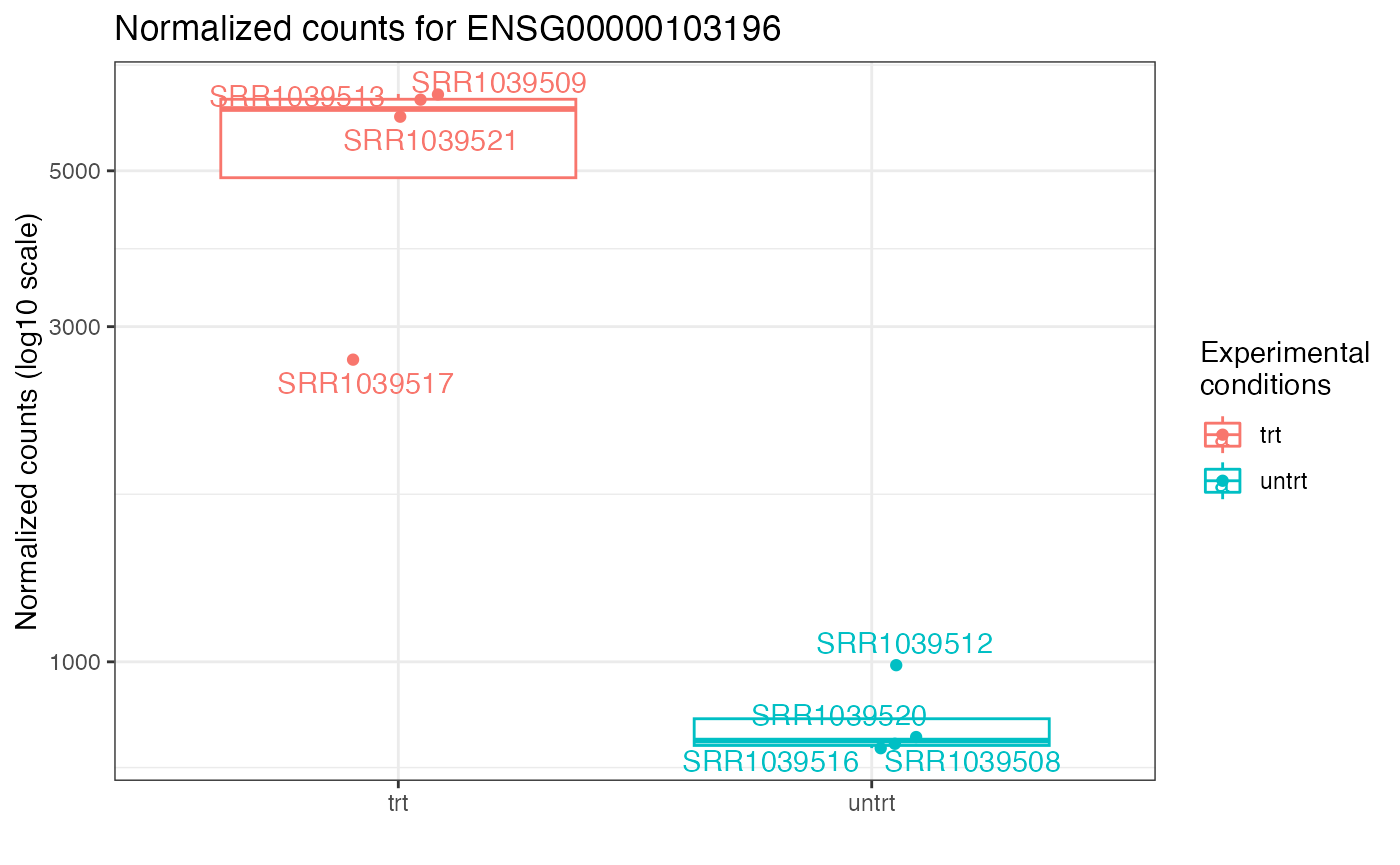
ggplotCounts
ggplotCounts extends the functionality of the
plotCounts function of DESeq2,
and plots the normalized counts of a single gene as a boxplot, with
jittered points superimposed.
ggplotCounts(
  dds = dds_airway,
  gene = "ENSG00000103196", # CRISPLD2 in the original publication
  intgroup = "dex"
)
If an annotation_obj is provided, their gene name can
also be included in the title.
ggplotCounts(
  dds = dds_airway,
  gene = "ENSG00000103196", # CRISPLD2 in the original publication
  intgroup = "dex",
  annotation_obj = annotation_airway
)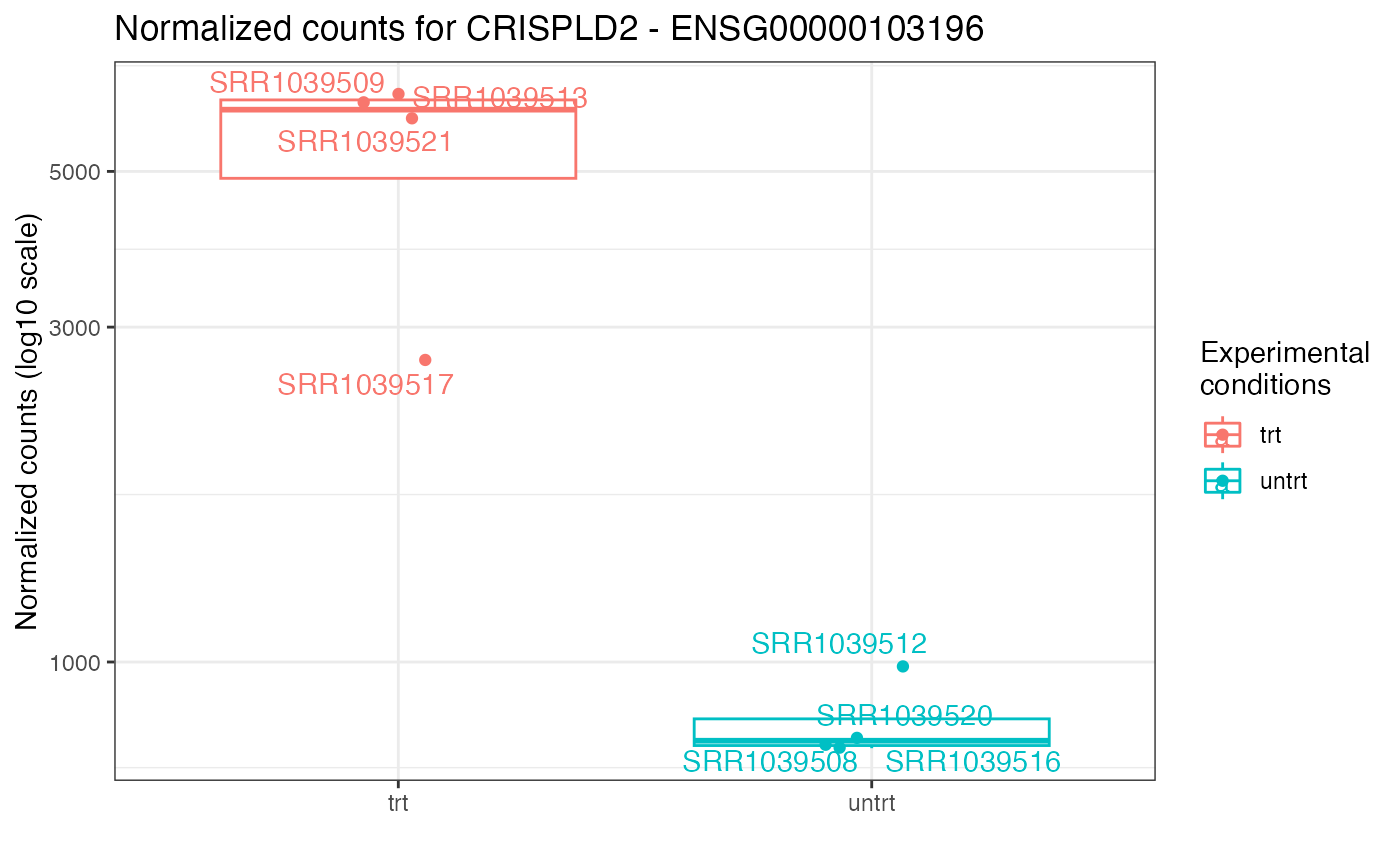
When used in the context of the app, it is possible to seamless search for genes also by their gene name, making exploration even more immediate.
From version 1.30.0 onwards, the ggplotCounts() function
has been deprecated, in favor of the equivalent
mosdef::gene_plot() function, which is more robust and
flexible in its usage.
goseqTable
goseqTable is a wrapper to extract the functional GO
terms enriched in in a list of (DE) genes, based on the algorithm and
the implementation in the goseq
package.
Its counterpart, based on the topGO package, can be found in the pcaExplorer package.
Please note that the following code chunks are not run only for reducing compilation time. The reader is invited to try out the functionality by simply executing these commands.
res_subset <- mosdef::deresult_to_df(res_airway)[1:100, ] # taking only a subset of the DE genes
myde <- res_subset$id
myassayed <- rownames(res_airway)
mygo <- goseqTable(
  de.genes = myde,
  assayed.genes = myassayed,
  genome = "hg38",
  id = "ensGene",
  testCats = "GO:BP",
  addGeneToTerms = FALSE
)
head(mygo)
As for the results, this table can be enhanced by adding the links for each category to the AmiGO database.
mygo_enhanced <- mygo
# using the unexported function to link the GO term to the entry in the AmiGO db
mygo_enhanced$category <- mosdef::create_link_GO(mygo_enhanced$category)
DT::datatable(mygo_enhanced, escape = FALSE)
From version 1.30.0 onwards, the goseqTable() function
has been deprecated, in favor of the equivalent
mosdef::run_goseq() function, which is faster, more robust
and flexible in its usage.
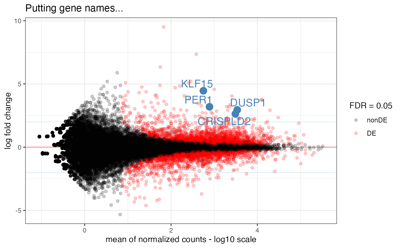
plot_ma
The MA plot provided by ideal
displays the gene-wise log2-fold changes (logFCs) versus the average
expression value. As a main input parameter, a DESeqResults
object is required. Control on the appearance of the plot can be applied
by selecting the False Discovery Rate (FDR), the point
transparency (point_alpha), adding horizontal lines at
particular logFC values (hlines). The user can also decide
to add rug plots in the margins (setting add_rug to
TRUE).
To facilitate the inspection of a particular gene or gene set,
intgenes can assume the value of a vector of genes (either
the IDs or the gene symbols if symbol column is provided in
res_obj. Labels can be added via
labels_intgenes, while classical labels/title can be also
edited as preferred (see plot_ma for all details).
plot_ma(res_airway,
  FDR = 0.05, hlines = 1,
  title = "Adding horizontal lines", add_rug = FALSE
)
plot_ma(res_airway,
  FDR = 0.1,
  intgenes = c(
    "ENSG00000103196", # CRISPLD2
    "ENSG00000120129", # DUSP1
    "ENSG00000163884", # KLF15
    "ENSG00000179094"
  ), # PER1
  title = "Providing a shortlist of genes",
  add_rug = FALSE
)
res_airway2 <- res_airway
res_airway2$symbol <- mapIds(org.Hs.eg.db, keys = rownames(res_airway2), column = "SYMBOL", keytype = "ENSEMBL")
#> 'select()' returned 1:many mapping between keys and columns
plot_ma(res_airway2,
  FDR = 0.05,
  intgenes = c(
    "CRISPLD2", # CRISPLD2
    "DUSP1", # DUSP1
    "KLF15", # KLF15
    "PER1"
  ), # PER1
  annotation_obj = annotation_airway,
  hlines = 2,
  add_rug = FALSE,
  title = "Putting gene names..."
)
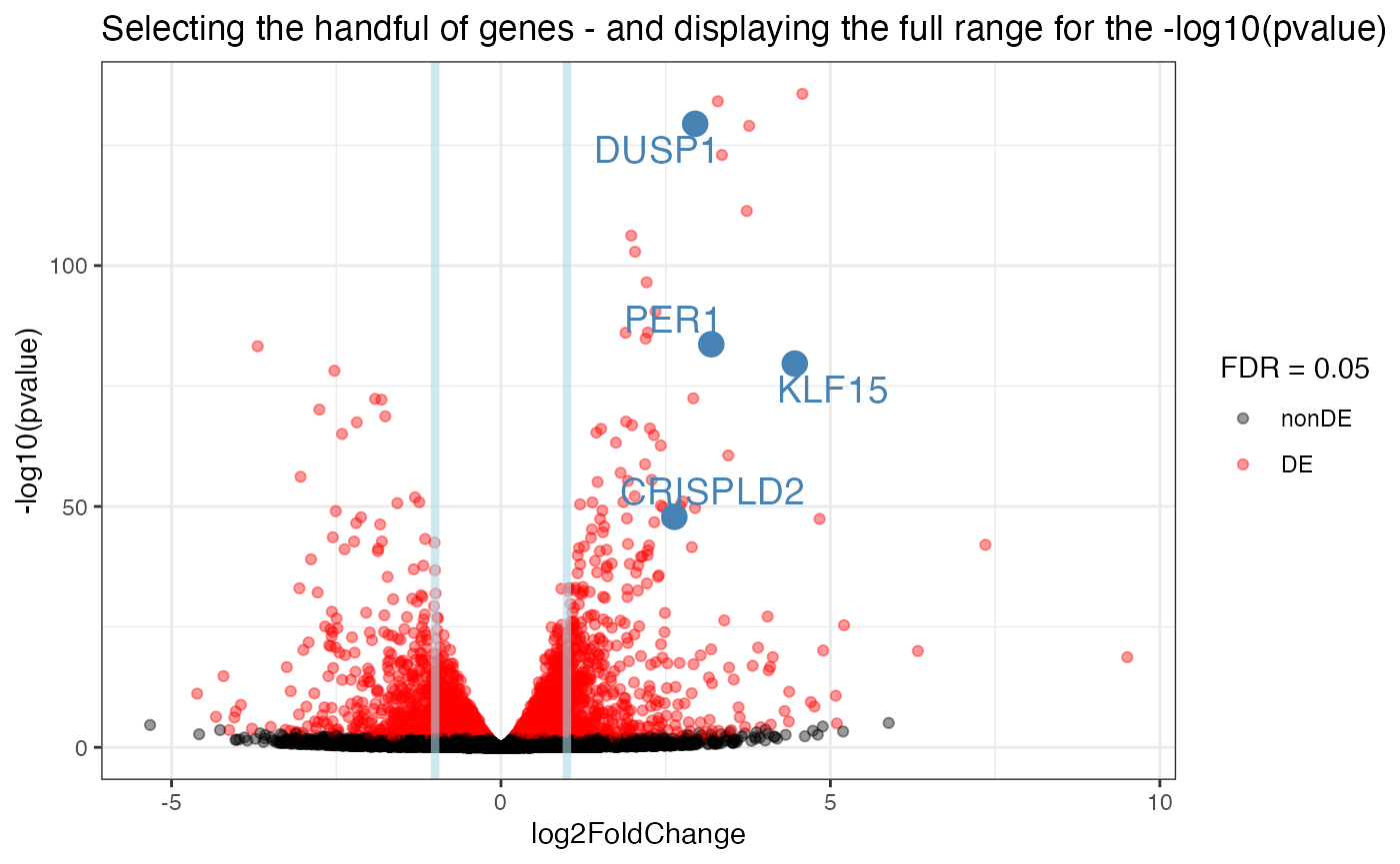
plot_volcano
The volcano plot gives a different flavor for the gene overview, displaying log2-fold changes and log p-values.
In a way similar to plot_ma, genes can be annotated with
intgenes, and vertical lines can be added via
vlines. ylim_up controls the y axis upper
limit to visualize better the bulk of genes - keep in mind that very
small p-values due to robust differences/large effect sizes can be “cut
out”.
plot_volcano(res_airway)
plot_volcano(res_airway2,
  FDR = 0.05,
  intgenes = c(
    "CRISPLD2", # CRISPLD2
    "DUSP1", # DUSP1
    "KLF15", # KLF15
    "PER1"
  ), # PER1
  title = "Selecting the handful of genes - and displaying the full range for the -log10(pvalue)",
  ylim_up = -log10(min(res_airway2$pvalue, na.rm = TRUE))
)
sepguesser
sepguesser makes an educated guess on the separator
character for the input text file (file). The separator
list can be provided as a vector in sep_list (defaults to
comma, tab, semicolon, and whitespace - which ideally could cover most
of the cases). The heuristics is based on the number of occurrencies of
each separator in each line.
sepguesser(system.file("extdata/design_commas.txt", package = "ideal"))#> [1] ","
sepguesser(system.file("extdata/design_semicolons.txt", package = "ideal"))#> [1] ";"
sepguesser(system.file("extdata/design_spaces.txt", package = "ideal"))#> [1] " "
anyfile <- system.file("extdata/design_tabs.txt", package = "ideal") # we know it is going to be TAB
guessed_sep <- sepguesser(anyfile)
guessed_sep
#> [1] "\t"
# to be used for reading in the same file, without having to specify the sep
read.delim(anyfile,
  header = TRUE, as.is = TRUE,
  sep = guessed_sep,
  quote = "", row.names = 1, check.names = FALSE
)
#> SampleName cell dex albut Run avgLength Experiment
#> SRR1039508 GSM1275862 N61311 untrt untrt SRR1039508 126 SRX384345
#> SRR1039509 GSM1275863 N61311 trt untrt SRR1039509 126 SRX384346
#> SRR1039512 GSM1275866 N052611 untrt untrt SRR1039512 126 SRX384349
#> SRR1039513 GSM1275867 N052611 trt untrt SRR1039513 87 SRX384350
#> SRR1039516 GSM1275870 N080611 untrt untrt SRR1039516 120 SRX384353
#> SRR1039517 GSM1275871 N080611 trt untrt SRR1039517 126 SRX384354
#> SRR1039520 GSM1275874 N061011 untrt untrt SRR1039520 101 SRX384357
#> SRR1039521 GSM1275875 N061011 trt untrt SRR1039521 98 SRX384358
#> Sample BioSample sizeFactor
#> SRR1039508 SRS508568 SAMN02422669 1.0236476
#> SRR1039509 SRS508567 SAMN02422675 0.8961667
#> SRR1039512 SRS508571 SAMN02422678 1.1794861
#> SRR1039513 SRS508572 SAMN02422670 0.6700538
#> SRR1039516 SRS508575 SAMN02422682 1.1776714
#> SRR1039517 SRS508576 SAMN02422673 1.3990365
#> SRR1039520 SRS508579 SAMN02422683 0.9207787
#> SRR1039521 SRS508580 SAMN02422677 0.9445141Creating and sharing output objects
While running the app, the user can
- generate and save graphics
- create and export tables
- generate, preview, download/export an HTML report
- save the values of the
reactiveValuesin an environment, or in binary format
This functionality to retrieve and share the output is provided by action buttons that are placed close to each element of interest.
Expanding the analysis after ideal
After exporting the objects to the R environment, via the button
“Exit ideal and save”, it is possible to continue the analyses
e.g. using alternative methods for functional enrichment analysis, with
Functional Class Scoring methods (such as GSEA, as implemented in fgsea), or
additional methods for Overrepresentation Analysis (e.g. gprofiler2).
In the example below, we show an example of the code required to perform
fgsea on the set of objects exported from
ideal().
library("fgsea")
# selecting the result object from the exported environment
exported_res <- ideal_env$ideal_values_20200926_135052$res_obj
summary(exported_res)

# for processing of intermediate steps
library("dplyr")
library("tibble")

# extracting the rankes for pre-ranked gsea
de_ranks <- exported_res %>%
  as.data.frame() %>%
  dplyr::arrange(padj) %>%
  dplyr::select(symbol, stat) %>%
  deframe()
head(de_ranks, 20)

# loading the signatures from the gmt file - to be downloaded locally
pathways_gmtfile <- gmtPathways("path_to/msigdb_v7.0_GMTs/h.all.v6.2.symbols.gmt")

# running fgsea
fgsea_result <- fgsea(
  pathways = pathways_gmtfile,
  stats = de_ranks,
  nperm = 100000
)
fgsea_result <- fgsea_result %>%
  arrange(desc(NES))

# displaying the results
DT::datatable(fgsea_result)
The following chunk shows an example of how to perform the functional
enrichment analysis with g:Profiler’s tool
g:GOST, using the interface in gprofiler2
library("gprofiler2")

# selecting the result object from the exported environment
exported_res <- ideal_env$ideal_values_20200926_135052$res_obj
summary(exported_res)

# extracting the DE genes vector
degenes <- deseqresult2DEgenes(exported_res, FDR = 0.01)$symbol

# running the test
gost_res <- gost(
  query = degenes[1:1000],
  organism = "hsapiens",
  ordered_query = FALSE,
  multi_query = FALSE,
  significant = FALSE,
  exclude_iea = TRUE,
  measure_underrepresentation = FALSE,
  evcodes = TRUE,
  user_threshold = 0.05,
  correction_method = "g_SCS",
  domain_scope = "annotated",
  numeric_ns = "",
  sources = "GO:BP",
  as_short_link = FALSE
)

# displaying the results
DT::datatable(gost_res$result)
Enhancing ideal
The annotation_obj is a quick helper to make your data
and results easier to read. For creating it, you can exploit the
corresponding org.XX.eg.db packages, available in
Bioconductor.
Currently available are the following (in alphabetical order):
- org.Ag.eg.db
- org.At.tair.db
- org.Bt.eg.db
- org.Ce.eg.db
- org.Cf.eg.db
- org.Dm.eg.db
- org.Dr.eg.db
- org.EcK12.eg.db
- org.EcSakai.eg.db
- org.Gg.eg.db
- org.Hs.eg.db
- org.Mm.eg.db
- org.Mmu.eg.db
- org.Pf.plasmo.db
- org.Pt.eg.db
- org.Rn.eg.db
- org.Sc.sgd.db
- org.Sco.eg.db
- org.Ss.eg.db
- org.Tgondii.eg.db
- org.Xl.eg.db
They can all be easily installed with
BiocManager::install("orgdb_packagename").
In a similar way, for using at best the goseq package,
the gene length information can also be computed if the corresponding
TxDb packages are installed. Currently, following
TxDb packages are available:
- TxDb.Athaliana.BioMart.plantsmart22
- TxDb.Athaliana.BioMart.plantsmart25
- TxDb.Athaliana.BioMart.plantsmart28
- TxDb.Btaurus.UCSC.bosTau8.refGene
- TxDb.Celegans.UCSC.ce11.refGene
- TxDb.Celegans.UCSC.ce6.ensGene
- TxDb.Cfamiliaris.UCSC.canFam3.refGene
- TxDb.Dmelanogaster.UCSC.dm3.ensGene
- TxDb.Dmelanogaster.UCSC.dm6.ensGene
- TxDb.Drerio.UCSC.danRer10.refGene
- TxDb.Ggallus.UCSC.galGal4.refGene
- TxDb.Hsapiens.UCSC.hg18.knownGene
- TxDb.Hsapiens.UCSC.hg19.knownGene
- TxDb.Hsapiens.UCSC.hg19.lincRNAsTranscripts
- TxDb.Hsapiens.UCSC.hg38.knownGene
- TxDb.Mmulatta.UCSC.rheMac3.refGene
- TxDb.Mmulatta.UCSC.rheMac8.refGene
- TxDb.Mmusculus.UCSC.mm10.ensGene
- TxDb.Mmusculus.UCSC.mm10.knownGene
- TxDb.Mmusculus.UCSC.mm9.knownGene
- TxDb.Ptroglodytes.UCSC.panTro4.refGene
- TxDb.Rnorvegicus.UCSC.rn4.ensGene
- TxDb.Rnorvegicus.UCSC.rn5.refGene
- TxDb.Rnorvegicus.UCSC.rn6.refGene
- TxDb.Scerevisiae.UCSC.sacCer2.sgdGene
- TxDb.Scerevisiae.UCSC.sacCer3.sgdGene
- TxDb.Sscrofa.UCSC.susScr3.refGene
As for the org.XX.eg.db above, these can all be quickly
installed with
BiocManager::install("txdb_packagename").
Further development
Additional functionality for the ideal will be added in the future, as it is tightly related to a topic under current development research.
Improvements, suggestions, bugs, issues and feedback of any type can be sent to marinif@uni-mainz.de.
Session Info
#> R version 4.5.0 (2025-04-11)
#> Platform: aarch64-apple-darwin20
#> Running under: macOS Sonoma 14.7.5
#>
#> Matrix products: default
#> BLAS:   /Library/Frameworks/R.framework/Versions/4.5-arm64/Resources/lib/libRblas.0.dylib
#> LAPACK: /Library/Frameworks/R.framework/Versions/4.5-arm64/Resources/lib/libRlapack.dylib;  LAPACK version 3.12.1
#>
#> locale:
#> [1] en_US.UTF-8/en_US.UTF-8/en_US.UTF-8/C/en_US.UTF-8/en_US.UTF-8
#>
#> time zone: UTC
#> tzcode source: internal
#>
#> attached base packages:
#> [1] stats4    stats     graphics  grDevices utils     datasets  methods
#> [8] base
#>
#> other attached packages:
#>  [1] edgeR_4.7.0                 limma_3.65.0
#>  [3] DEFormats_1.37.0            org.Hs.eg.db_3.21.0
#>  [5] DESeq2_1.49.0               airway_1.29.0
#>  [7] SummarizedExperiment_1.39.0 GenomicRanges_1.61.0
#>  [9] GenomeInfoDb_1.45.3         MatrixGenerics_1.21.0
#> [11] matrixStats_1.5.0           ideal_2.3.0
#> [13] topGO_2.59.0                SparseM_1.84-2
#> [15] GO.db_3.21.0                AnnotationDbi_1.71.0
#> [17] IRanges_2.43.0              S4Vectors_0.47.0
#> [19] Biobase_2.69.0              graph_1.87.0
#> [21] BiocGenerics_0.55.0         generics_0.1.3
#> [23] knitr_1.50                  BiocStyle_2.37.0
#>
#> loaded via a namespace (and not attached):
#>   [1] fs_1.6.6                 bitops_1.0-9             enrichplot_1.29.1
#>   [4] fontawesome_0.5.3        httr_1.4.7               webshot_0.5.5
#>   [7] RColorBrewer_1.1-3       Rgraphviz_2.53.0         backports_1.5.0
#>  [10] tools_4.5.0              R6_2.6.1                 DT_0.33
#>  [13] lazyeval_0.2.2           mgcv_1.9-3               withr_3.0.2
#>  [16] prettyunits_1.2.0        gridExtra_2.3            fdrtool_1.2.18
#>  [19] cli_3.6.5                textshaping_1.0.1        TSP_1.2-4
#>  [22] labeling_0.4.3           slam_0.1-55              sass_0.4.10
#>  [25] genefilter_1.91.0        goseq_1.61.0             pkgdown_2.1.2.9000
#>  [28] Rsamtools_2.25.0         systemfonts_1.2.3        yulab.utils_0.2.0
#>  [31] gson_0.1.0               txdbmaker_1.5.0          DOSE_4.3.0
#>  [34] R.utils_2.13.0           rentrez_1.2.3            AnnotationForge_1.51.0
#>  [37] RSQLite_2.3.9            GOstats_2.75.0           gridGraphics_0.5-1
#>  [40] BiocIO_1.19.0            crosstalk_1.2.1          gtools_3.9.5
#>  [43] dplyr_1.1.4              dendextend_1.19.0        Matrix_1.7-3
#>  [46] abind_1.4-8              R.methodsS3_1.8.2        lifecycle_1.0.4
#>  [49] yaml_2.3.10              gplots_3.2.0             qvalue_2.41.0
#>  [52] SparseArray_1.9.0        BiocFileCache_2.99.0     grid_4.5.0
#>  [55] blob_1.2.4               promises_1.3.2           crayon_1.5.3
#>  [58] shinydashboard_0.7.3     ggtangle_0.0.6           lattice_0.22-7
#>  [61] cowplot_1.1.3            annotate_1.87.0          GenomicFeatures_1.61.0
#>  [64] KEGGREST_1.49.0          pillar_1.10.2            fgsea_1.35.0
#>  [67] rjson_0.2.23             codetools_0.2-20         fastmatch_1.1-6
#>  [70] glue_1.8.0               ggfun_0.1.8              data.table_1.17.0
#>  [73] vctrs_0.6.5              png_0.1-8                treeio_1.33.0
#>  [76] gtable_0.3.6             assertthat_0.2.1         cachem_1.1.0
#>  [79] xfun_0.52                S4Arrays_1.9.0           mime_0.13
#>  [82] survival_3.8-3           pheatmap_1.0.12          seriation_1.5.7
#>  [85] iterators_1.0.14         statmod_1.5.0            Category_2.75.0
#>  [88] nlme_3.1-168             ggtree_3.17.0            bit64_4.6.0-1
#>  [91] progress_1.2.3           filelock_1.0.3           UpSetR_1.4.0
#>  [94] bslib_0.9.0              KernSmooth_2.23-26       colorspace_2.1-1
#>  [97] DBI_1.2.3                tidyselect_1.2.1         bit_4.6.0
#> [100] compiler_4.5.0           curl_6.2.2               httr2_1.1.2
#> [103] BiasedUrn_2.0.12         xml2_1.3.8               desc_1.4.3
#> [106] DelayedArray_0.35.1      plotly_4.10.4            bookdown_0.43
#> [109] rtracklayer_1.69.0       checkmate_2.3.2          scales_1.4.0
#> [112] caTools_1.18.3           mosdef_1.3.1             RBGL_1.85.0
#> [115] rappdirs_0.3.3           stringr_1.5.1            digest_0.6.37
#> [118] shinyBS_0.61.1           rmarkdown_2.29           ca_0.71.1
#> [121] XVector_0.49.0           htmltools_0.5.8.1        pkgconfig_2.0.3
#> [124] base64enc_0.1-3          lpsymphony_1.37.0        dbplyr_2.5.0
#> [127] fastmap_1.2.0            rlang_1.1.6              htmlwidgets_1.6.4
#> [130] UCSC.utils_1.5.0         shiny_1.10.0             farver_2.1.2
#> [133] jquerylib_0.1.4          IHW_1.37.0               jsonlite_2.0.0
#> [136] BiocParallel_1.43.0      GOSemSim_2.35.0          R.oo_1.27.0
#> [139] RCurl_1.98-1.17          magrittr_2.0.3           ggplotify_0.1.2
#> [142] patchwork_1.3.0          Rcpp_1.0.14              ape_5.8-1
#> [145] viridis_0.6.5            rintrojs_0.3.4           stringi_1.8.7
#> [148] MASS_7.3-65              plyr_1.8.9               parallel_4.5.0
#> [151] ggrepel_0.9.6            Biostrings_2.77.0        splines_4.5.0
#> [154] hms_1.1.3                geneLenDataBase_1.45.0   locfit_1.5-9.12
#> [157] igraph_2.1.4             reshape2_1.4.4           biomaRt_2.65.0
#> [160] XML_3.99-0.18            evaluate_1.0.3           BiocManager_1.30.25
#> [163] foreach_1.5.2            tweenr_2.0.3             httpuv_1.6.16
#> [166] tidyr_1.3.1              purrr_1.0.4              polyclip_1.10-7
#> [169] heatmaply_1.5.0          ggplot2_3.5.2            ggforce_0.4.2
#> [172] xtable_1.8-4             restfulr_0.0.15          tidytree_0.4.6
#> [175] later_1.4.2              viridisLite_0.4.2        ragg_1.4.0
#> [178] tibble_3.2.1             clusterProfiler_4.17.0   aplot_0.2.5
#> [181] memoise_2.0.1            registry_0.5-1           GenomicAlignments_1.45.0
#> [184] GSEABase_1.71.0          shinyAce_0.4.4