Introduction
Method benchmarking is a core part of computational biology research, with an intrinsic power to establish best practices in method selection and application, as well as help identifying gaps and possibilities for improvement. A typical benchmark evaluates a set of methods using multiple different metrics, intended to capture different aspects of their performance. The best method to choose in any given situation can then be found, e.g., by averaging the different performance metrics, possibly putting more emphasis on those that are more important to the specific situation.
Inspired by the OECD ‘Better
Life Index’, the bettr package was developed to provide
support for this last step. It allows users to easily create performance
summaries emphasizing the aspects that are most important to them.
bettr can be used interactively, via a R/Shiny application,
or programmatically by calling the underlying functions. In this
vignette, we illustrate both alternatives, using example data provided
with the package.
Given the abundance of methods available for computational analysis
of biological data, both within and beyond Bioconductor, and the
importance of careful, adaptive benchmarking, we believe that
bettr will be a useful complement to currently available
Bioconductor infrastructure related to benchmarking and performance
estimation. Other packages (e.g., pipeComp)
provide frameworks for executing benchmarks by applying and
recording pre-defined workflows to data. Packages such as iCOBRA and
ROCR
instead provide functionality for calculating well-established
evaluation metrics. In contrast, bettr focuses on
visual exploration of benchmark results, represented by the
values of several evaluation metrics.
Installation
bettr can be installed from Bioconductor (from release
3.19 onwards):
if (!require("BiocManager", quietly = TRUE))
    install.packages("BiocManager")

BiocManager::install("bettr")
Usage
suppressPackageStartupMessages({
    library("bettr")
    library("SummarizedExperiment")
    library("tibble")
    library("dplyr")
})
The main input to bettr is a data.frame
containing values of several metrics for several methods. In addition,
the user can provide additional annotations and characteristics for the
methods and metrics, which can be used to group and filter them in the
interactive application.
## Data for two metrics (metric1, metric2) for three methods (M1, M2, M3)
df <- data.frame(Method = c("M1", "M2", "M3"),
                 metric1 = c(1.0, 2.0, 3.0),
                 metric2 = c(3.0, 1.0, 2.0))

## More information for metrics
metricInfo <- data.frame(Metric = c("metric1", "metric2", "metric3"),
                         Group = c("G1", "G2", "G2"))

## More information for methods ('IDs')
idInfo <- data.frame(Method = c("M1", "M2", "M3"),
                     Type = c("T1", "T1", "T2"))
To simplify handling and sharing, the data can be combined into a
SummarizedExperiment object (with methods as rows and
metrics as columns) as follows:
se <- assembleSE(df = df, idCol = "Method", metricInfo = metricInfo,
                 idInfo = idInfo)
se
#> class: SummarizedExperiment
#> dim: 3 2
#> metadata(1): bettrInfo
#> assays(1): values
#> rownames(3): M1 M2 M3
#> rowData names(2): Method Type
#> colnames(2): metric1 metric2
#> colData names(2): Metric Group
The interactive application to explore the rankings can then be
launched by calling the bettr() function. The input can be
either the assembled SummarizedExperiment object or the
individual components.
Example - single-cell RNA-seq clustering benchmark
Next, we show a more elaborate example, visualizing data from the
benchmark of single-cell clustering methods performed by Duo et al (2018).
The values for a set of evaluation metrics applied to results obtained
by several clustering methods are provided in a .csv file
in the package:
res <- read.csv(system.file("extdata", "duo2018_results.csv",
                            package = "bettr"))
dim(res)
#> [1] 14 49
tibble(res)
#> # A tibble: 14 × 49
#>    method      ARI_Koh ARI_KohTCC ARI_Kumar ARI_KumarTCC ARI_SimKumar4easy
#>    <chr>         <dbl>      <dbl>     <dbl>        <dbl>             <dbl>
#>  1 CIDR          0.672      0.805     0.989        0.977             1
#>  2 FlowSOM       0.699      0.855     0.512        0.563             1
#>  3 PCAHC         0.869      0.891     1            1                 1
#>  4 PCAKmeans     0.836      0.903     0.989        0.978             1
#>  5 RaceID2       0.280      0.276     0.949        1                 0.644
#>  6 RtsneKmeans   0.966      0.967     0.989        1                 1
#>  7 SAFE          0.613      0.950     0.989        1                 0.952
#>  8 SC3           0.939      0.939     1            1                 1
#>  9 SC3svm        0.927      0.929     1            1                 1
#> 10 Seurat        0.862      0.902     0.988        0.989             1
#> 11 TSCAN         0.639      0.618     1            1                 1
#> 12 monocle       0.855      0.963     0.988        1                 0.995
#> 13 pcaReduce     0.935      0.979     1            1                 1
#> 14 ascend       NA         NA         1            0.988             1
#> # ℹ 43 more variables: ARI_SimKumar4hard <dbl>, ARI_SimKumar8hard <dbl>,
#> #   ARI_Trapnell <dbl>, ARI_TrapnellTCC <dbl>, ARI_Zhengmix4eq <dbl>,
#> #   ARI_Zhengmix4uneq <dbl>, ARI_Zhengmix8eq <dbl>, elapsed_Koh <dbl>,
#> #   elapsed_KohTCC <dbl>, elapsed_Kumar <dbl>, elapsed_KumarTCC <dbl>,
#> #   elapsed_SimKumar4easy <dbl>, elapsed_SimKumar4hard <dbl>,
#> #   elapsed_SimKumar8hard <dbl>, elapsed_Trapnell <dbl>,
#> #   elapsed_TrapnellTCC <dbl>, elapsed_Zhengmix4eq <dbl>, …
As we can see, we have 14 methods (rows) and 48 different metrics
(columns). The first column provides the name of the clustering method.
More precisely, the columns correspond to four different metrics, each
of which was applied to clustering output from 12 data sets. We encode
this “grouping” of metrics in a data frame, in such a way that we can
later collapse performance across data sets in bettr:
metricInfo <- tibble(Metric = colnames(res)[-1L]) |>
    mutate(Class = sub("_.*", "", Metric))
head(metricInfo)
#> # A tibble: 6 × 2
#>   Metric            Class
#>   <chr>             <chr>
#> 1 ARI_Koh           ARI
#> 2 ARI_KohTCC        ARI
#> 3 ARI_Kumar         ARI
#> 4 ARI_KumarTCC      ARI
#> 5 ARI_SimKumar4easy ARI
#> 6 ARI_SimKumar4hard ARI
table(metricInfo$Class)
#>
#>            ARI        elapsed nclust.vs.true s.norm.vs.true
#>             12             12             12             12
In order to make different metrics comparable, we next define the
transformation that should be applied to each of them within
bettr. First, we need to make sure that the metric are
consistent in terms of whether large values indicate “good” or “bad”
performance. In our case, for both the elapsed (elapsed run
time), nclust.vs.true (difference between estimated and
true number of clusters) and s.norm.vs.true (difference
between estimated and true normalized Shannon entropy for a clustering),
a small value indicates “better” performance, while for the
ARI (adjusted Rand index), larger values are better. Hence,
we will flip the sign of the first three before doing additional
analyses. Moreover, the different metrics clearly live in different
numeric ranges - the maximal value of the ARI is 1, while
the other metrics can have much larger values. As an example, here we
therefore scale the three other metrics linearly to the interval
[0, 1] to make them more comparable to the ARI
values. We record these transformations in a list, that will be passed
to bettr:
## Initialize list
initialTransforms <- lapply(res[, grep("elapsed|nclust.vs.true|s.norm.vs.true",
                                       colnames(res), value = TRUE)],
                            function(i) {
                                list(flip = TRUE, transform = "[0,1]")
                            })

length(initialTransforms)
#> [1] 36
names(initialTransforms)
#>  [1] "elapsed_Koh"                  "elapsed_KohTCC"
#>  [3] "elapsed_Kumar"                "elapsed_KumarTCC"
#>  [5] "elapsed_SimKumar4easy"        "elapsed_SimKumar4hard"
#>  [7] "elapsed_SimKumar8hard"        "elapsed_Trapnell"
#>  [9] "elapsed_TrapnellTCC"          "elapsed_Zhengmix4eq"
#> [11] "elapsed_Zhengmix4uneq"        "elapsed_Zhengmix8eq"
#> [13] "s.norm.vs.true_Koh"           "s.norm.vs.true_KohTCC"
#> [15] "s.norm.vs.true_Kumar"         "s.norm.vs.true_KumarTCC"
#> [17] "s.norm.vs.true_SimKumar4easy" "s.norm.vs.true_SimKumar4hard"
#> [19] "s.norm.vs.true_SimKumar8hard" "s.norm.vs.true_Trapnell"
#> [21] "s.norm.vs.true_TrapnellTCC"   "s.norm.vs.true_Zhengmix4eq"
#> [23] "s.norm.vs.true_Zhengmix4uneq" "s.norm.vs.true_Zhengmix8eq"
#> [25] "nclust.vs.true_Koh"           "nclust.vs.true_KohTCC"
#> [27] "nclust.vs.true_Kumar"         "nclust.vs.true_KumarTCC"
#> [29] "nclust.vs.true_SimKumar4easy" "nclust.vs.true_SimKumar4hard"
#> [31] "nclust.vs.true_SimKumar8hard" "nclust.vs.true_Trapnell"
#> [33] "nclust.vs.true_TrapnellTCC"   "nclust.vs.true_Zhengmix4eq"
#> [35] "nclust.vs.true_Zhengmix4uneq" "nclust.vs.true_Zhengmix8eq"
head(initialTransforms)
#> $elapsed_Koh
#> $elapsed_Koh$flip
#> [1] TRUE
#>
#> $elapsed_Koh$transform
#> [1] "[0,1]"
#>
#>
#> $elapsed_KohTCC
#> $elapsed_KohTCC$flip
#> [1] TRUE
#>
#> $elapsed_KohTCC$transform
#> [1] "[0,1]"
#>
#>
#> $elapsed_Kumar
#> $elapsed_Kumar$flip
#> [1] TRUE
#>
#> $elapsed_Kumar$transform
#> [1] "[0,1]"
#>
#>
#> $elapsed_KumarTCC
#> $elapsed_KumarTCC$flip
#> [1] TRUE
#>
#> $elapsed_KumarTCC$transform
#> [1] "[0,1]"
#>
#>
#> $elapsed_SimKumar4easy
#> $elapsed_SimKumar4easy$flip
#> [1] TRUE
#>
#> $elapsed_SimKumar4easy$transform
#> [1] "[0,1]"
#>
#>
#> $elapsed_SimKumar4hard
#> $elapsed_SimKumar4hard$flip
#> [1] TRUE
#>
#> $elapsed_SimKumar4hard$transform
#> [1] "[0,1]"
We can specify four different aspects of the desired transform, which will be applied in the following order:
-
flip(TRUEorFALSE, whether to flip the sign of the values). The default isFALSE. -
offset(a numeric value to add to the observed values, possibly after applying the sign flip). The default is 0. -
transform(one ofNone,[0,1],[-1,1],z-score, orRank). The default isNone. -
cuts(a numeric vector of cuts that will be used to turn a numeric variable into a categorical one). The default isNULL.
Only values that deviate from the defaults need to be specified.
Finally, we can define a set of colors that we would like to use for
visualizing the methods and metrics in bettr.
metricColors <- list(
    Class = c(ARI = "purple", elapsed = "forestgreen",
              nclust.vs.true = "blue",
              s.norm.vs.true = "orange")
)
idColors <- list(
    method = c(
        CIDR = "#332288", FlowSOM = "#6699CC", PCAHC = "#88CCEE",
        PCAKmeans = "#44AA99", pcaReduce = "#117733",
        RtsneKmeans = "#999933", Seurat = "#DDCC77", SC3svm = "#661100",
        SC3 = "#CC6677", TSCAN = "grey34", ascend = "orange", SAFE = "black",
        monocle = "red", RaceID2 = "blue"
    )
)
All the information defined so far can be combined in a
SummarizedExperiment object, as shown above for the small
example data:
duo2018 <- assembleSE(df = res, idCol = "method", metricInfo = metricInfo,
                      initialTransforms = initialTransforms,
                      metricColors = metricColors, idColors = idColors)
duo2018
#> class: SummarizedExperiment
#> dim: 14 48
#> metadata(1): bettrInfo
#> assays(1): values
#> rownames(14): CIDR FlowSOM ... pcaReduce ascend
#> rowData names(0):
#> colnames(48): ARI_Koh ARI_KohTCC ... nclust.vs.true_Zhengmix4uneq
#>   nclust.vs.true_Zhengmix8eq
#> colData names(2): Metric Class
The assay of the SummarizedExperiment
object contains the values for the 48 performance measures for the 14
clustering methods. The metricInfo is stored in the
colData, and the lists of colors and the initial transforms
in the metadata:
## Display the whole performance table
tibble(assay(duo2018, "values"))
#> # A tibble: 14 × 48
#>    ARI_Koh ARI_KohTCC ARI_Kumar ARI_KumarTCC ARI_SimKumar4easy ARI_SimKumar4hard
#>      <dbl>      <dbl>     <dbl>        <dbl>             <dbl>             <dbl>
#>  1   0.672      0.805     0.989        0.977             1                 1
#>  2   0.699      0.855     0.512        0.563             1                 1
#>  3   0.869      0.891     1            1                 1                 1
#>  4   0.836      0.903     0.989        0.978             1                 1
#>  5   0.280      0.276     0.949        1                 0.644             0.194
#>  6   0.966      0.967     0.989        1                 1                 1
#>  7   0.613      0.950     0.989        1                 0.952            NA
#>  8   0.939      0.939     1            1                 1                 1
#>  9   0.927      0.929     1            1                 1                 1
#> 10   0.862      0.902     0.988        0.989             1                 1
#> 11   0.639      0.618     1            1                 1                 1
#> 12   0.855      0.963     0.988        1                 0.995             0.992
#> 13   0.935      0.979     1            1                 1                 1
#> 14  NA         NA         1            0.988             1                 1
#> # ℹ 42 more variables: ARI_SimKumar8hard <dbl>, ARI_Trapnell <dbl>,
#> #   ARI_TrapnellTCC <dbl>, ARI_Zhengmix4eq <dbl>, ARI_Zhengmix4uneq <dbl>,
#> #   ARI_Zhengmix8eq <dbl>, elapsed_Koh <dbl>, elapsed_KohTCC <dbl>,
#> #   elapsed_Kumar <dbl>, elapsed_KumarTCC <dbl>, elapsed_SimKumar4easy <dbl>,
#> #   elapsed_SimKumar4hard <dbl>, elapsed_SimKumar8hard <dbl>,
#> #   elapsed_Trapnell <dbl>, elapsed_TrapnellTCC <dbl>,
#> #   elapsed_Zhengmix4eq <dbl>, elapsed_Zhengmix4uneq <dbl>, …

## Showing the first metric, evaluated on all datasets
head(colData(duo2018), 12L)
#> DataFrame with 12 rows and 2 columns
#>                              Metric       Class
#>                         <character> <character>
#> ARI_Koh                     ARI_Koh         ARI
#> ARI_KohTCC               ARI_KohTCC         ARI
#> ARI_Kumar                 ARI_Kumar         ARI
#> ARI_KumarTCC           ARI_KumarTCC         ARI
#> ARI_SimKumar4easy ARI_SimKumar4easy         ARI
#> ...                             ...         ...
#> ARI_Trapnell           ARI_Trapnell         ARI
#> ARI_TrapnellTCC     ARI_TrapnellTCC         ARI
#> ARI_Zhengmix4eq     ARI_Zhengmix4eq         ARI
#> ARI_Zhengmix4uneq ARI_Zhengmix4uneq         ARI
#> ARI_Zhengmix8eq     ARI_Zhengmix8eq         ARI

## These are the color definitions (can mix character and hex values)
metadata(duo2018)$bettrInfo$idColors
#> $method
#>        CIDR     FlowSOM       PCAHC   PCAKmeans   pcaReduce RtsneKmeans
#>   "#332288"   "#6699CC"   "#88CCEE"   "#44AA99"   "#117733"   "#999933"
#>      Seurat      SC3svm         SC3       TSCAN      ascend        SAFE
#>   "#DDCC77"   "#661100"   "#CC6677"    "grey34"    "orange"     "black"
#>     monocle     RaceID2
#>       "red"      "blue"
metadata(duo2018)$bettrInfo$metricColors
#> $Class
#>            ARI        elapsed nclust.vs.true s.norm.vs.true
#>       "purple"  "forestgreen"         "blue"       "orange"

names(metadata(duo2018)$bettrInfo$initialTransforms)
#>  [1] "elapsed_Koh"                  "elapsed_KohTCC"
#>  [3] "elapsed_Kumar"                "elapsed_KumarTCC"
#>  [5] "elapsed_SimKumar4easy"        "elapsed_SimKumar4hard"
#>  [7] "elapsed_SimKumar8hard"        "elapsed_Trapnell"
#>  [9] "elapsed_TrapnellTCC"          "elapsed_Zhengmix4eq"
#> [11] "elapsed_Zhengmix4uneq"        "elapsed_Zhengmix8eq"
#> [13] "s.norm.vs.true_Koh"           "s.norm.vs.true_KohTCC"
#> [15] "s.norm.vs.true_Kumar"         "s.norm.vs.true_KumarTCC"
#> [17] "s.norm.vs.true_SimKumar4easy" "s.norm.vs.true_SimKumar4hard"
#> [19] "s.norm.vs.true_SimKumar8hard" "s.norm.vs.true_Trapnell"
#> [21] "s.norm.vs.true_TrapnellTCC"   "s.norm.vs.true_Zhengmix4eq"
#> [23] "s.norm.vs.true_Zhengmix4uneq" "s.norm.vs.true_Zhengmix8eq"
#> [25] "nclust.vs.true_Koh"           "nclust.vs.true_KohTCC"
#> [27] "nclust.vs.true_Kumar"         "nclust.vs.true_KumarTCC"
#> [29] "nclust.vs.true_SimKumar4easy" "nclust.vs.true_SimKumar4hard"
#> [31] "nclust.vs.true_SimKumar8hard" "nclust.vs.true_Trapnell"
#> [33] "nclust.vs.true_TrapnellTCC"   "nclust.vs.true_Zhengmix4eq"
#> [35] "nclust.vs.true_Zhengmix4uneq" "nclust.vs.true_Zhengmix8eq"

## An example of a transformation - elapsed time for the Koh dataset
metadata(duo2018)$bettrInfo$initialTransforms$elapsed_Koh
#> $flip
#> [1] TRUE
#>
#> $transform
#> [1] "[0,1]"
Now, we can launch the app for this data set:
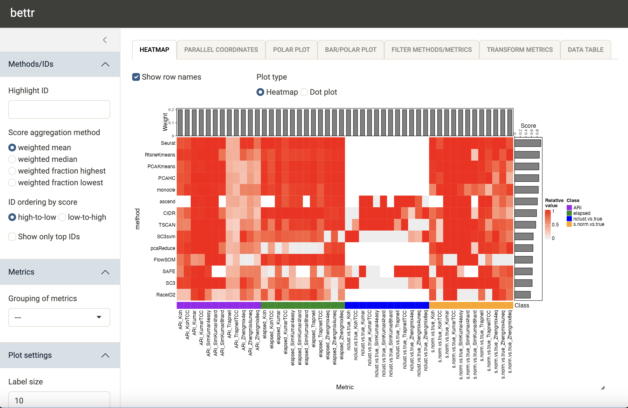
bettr(bettrSE = duo2018, bstheme = "sandstone")The screenshot below illustrates the default view of the interactive
interface. The methods (rows) are sorted by the aggregated scores, which
are shown as bars to the right of the heatmap (recall that in this case,
large scores are better). If we have many methods, we can choose to only
display the top ones by ticking the Show only top IDs box
in the left-hand sidebar. If additional annotations are provided for the
methods (similarly as for the metrics above), we can further display
only the top methods in each group. This can be useful e.g. in
situations where each tool is run with many different parameter
settings, and we want to limit the plot to the best parameter settings
for each tool.
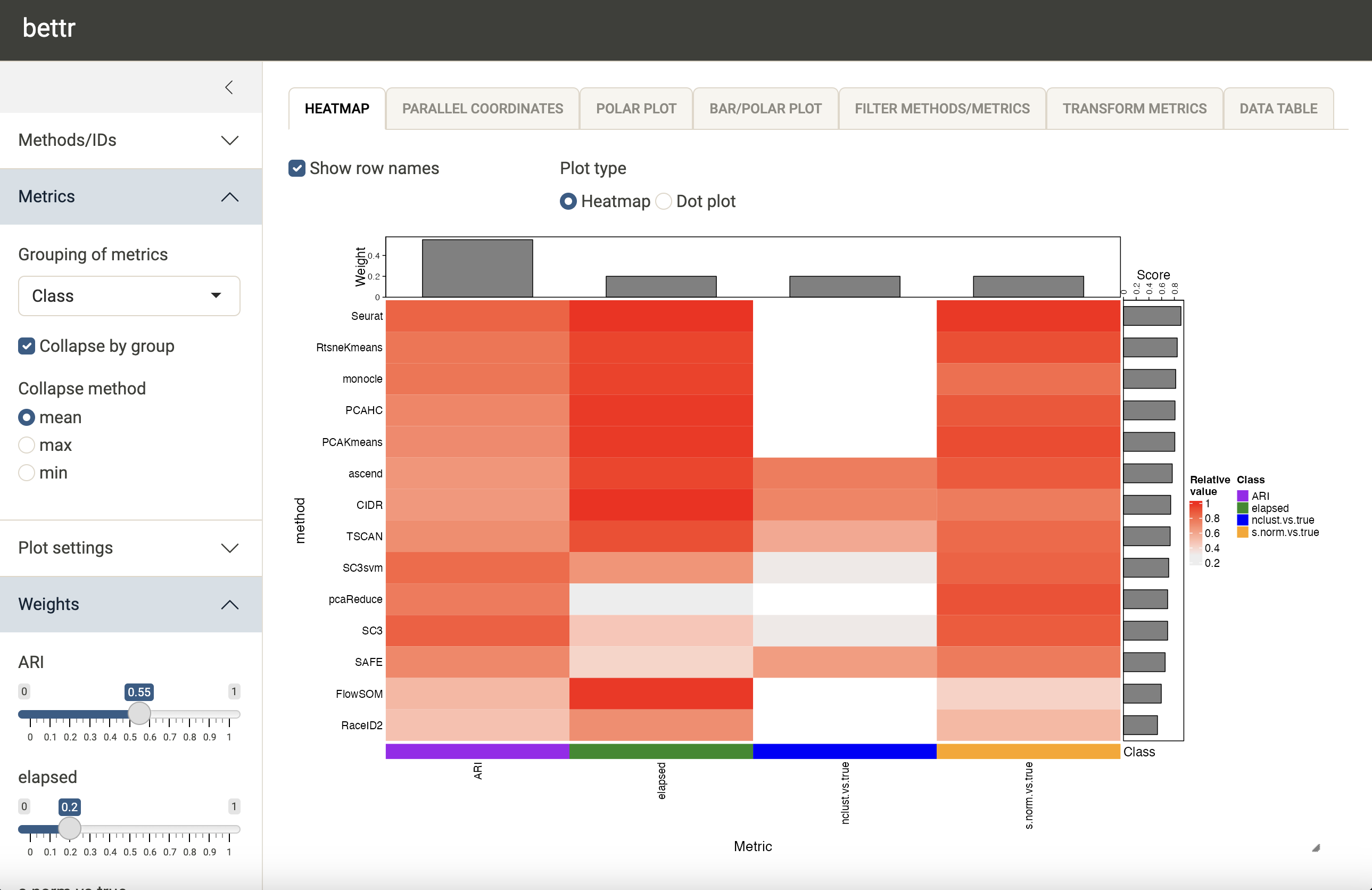
We can choose to collapse the metric values to have a single value
for each metric class, to reduce the redundancy (via
Metrics - Grouping of metrics in the left-hand
sidebar). We can now also freely decide how to weight the respective
metrics by means of the sliders in the left side bar. The bars on top of
the heatmap show the current weight assignment.
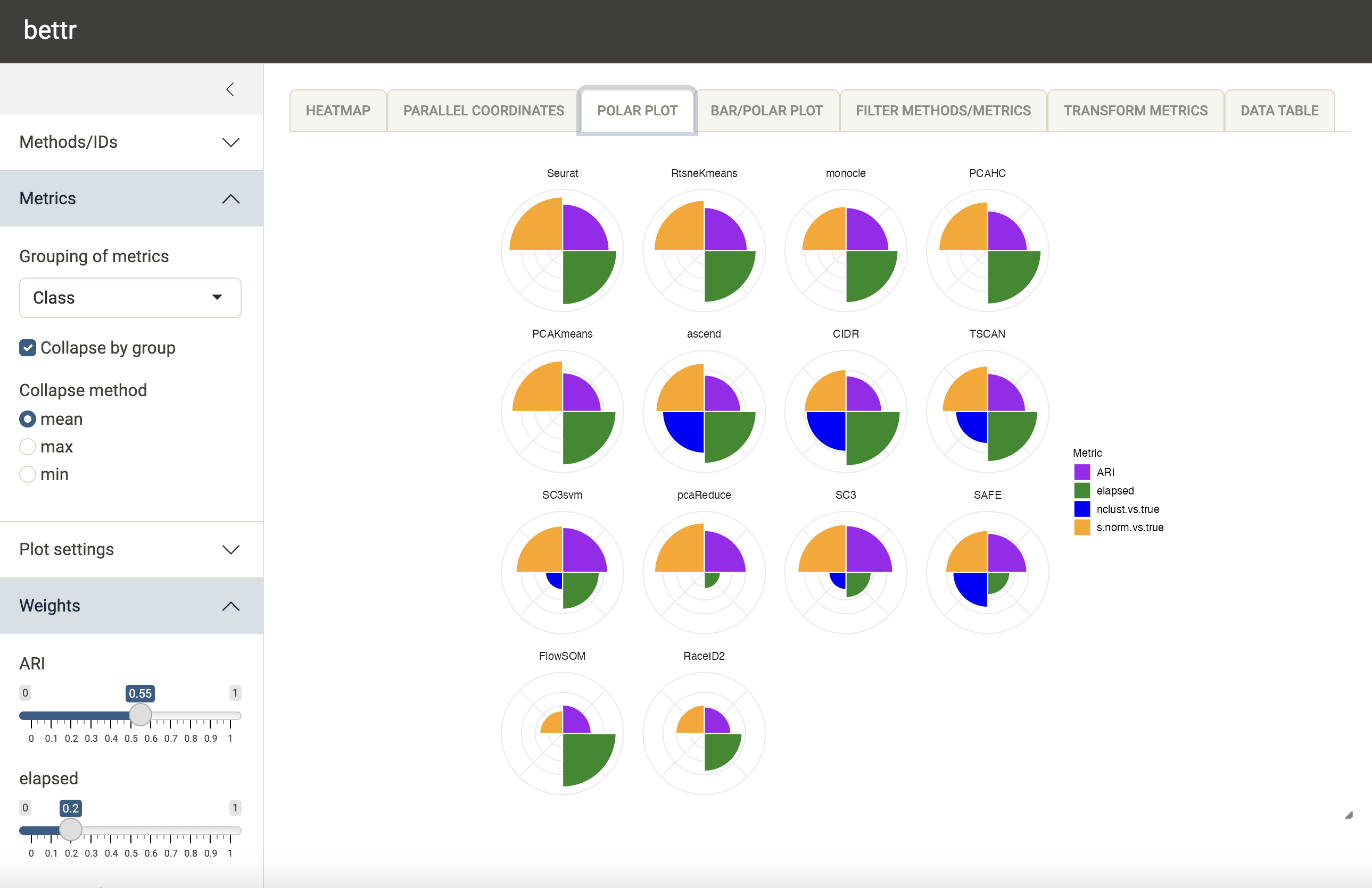
bettr also provides alternative visualizations, e.g. a
polar plot:
At any point, methods and metrics can be filtered out (either
individually or by excluding all methods and metrics with a specified
annotation) via the Filter methods/metrics tab. The metrics
can be transformed interactively in the Transform metrics
tab (see above for the different transformation options). Finally, the
current transformed values for all metrics as well as the summary scores
can be viewed in the Data table tab.
Programmatic interface
The interactive application showcased above is the main entry point
to using bettr. However, we also provide a wrapper function
to prepare the input data for plotting (replicating the steps that are
performed in the app), as well as access to the plotting functions
themselves. The following code replicates the results for the example
above.
## Assign a higher weight to one of the collapsed metric classes
metadata(duo2018)$bettrInfo$initialWeights["Class_ARI"] <- 0.55

prepData <- bettrGetReady(
    bettrSE = duo2018, idCol = "method",
    scoreMethod = "weighted mean", metricGrouping = "Class",
    metricCollapseGroup = TRUE
)

## This object is fairly verbose and detailed,
## but has the whole set of info needed
prepData
#> $plotdata
#>         method    metricGroup ScaledValue Weight         Metric
#> 1         CIDR            ARI   0.6512593   0.55            ARI
#> 2         CIDR        elapsed   0.9889737   0.20        elapsed
#> 3         CIDR nclust.vs.true   0.7250000   0.20 nclust.vs.true
#> 4         CIDR s.norm.vs.true   0.7637276   0.20 s.norm.vs.true
#> 5      FlowSOM            ARI   0.5211600   0.55            ARI
#> 6      FlowSOM        elapsed   0.9743747   0.20        elapsed
#> 7      FlowSOM nclust.vs.true          NA   0.20 nclust.vs.true
#> 8      FlowSOM s.norm.vs.true   0.4148342   0.20 s.norm.vs.true
#> 9        PCAHC            ARI   0.7226564   0.55            ARI
#> 10       PCAHC        elapsed   0.9737352   0.20        elapsed
#> 11       PCAHC nclust.vs.true          NA   0.20 nclust.vs.true
#> 12       PCAHC s.norm.vs.true   0.8884335   0.20 s.norm.vs.true
#> 13   PCAKmeans            ARI   0.7046547   0.55            ARI
#> 14   PCAKmeans        elapsed   0.9725792   0.20        elapsed
#> 15   PCAKmeans nclust.vs.true          NA   0.20 nclust.vs.true
#> 16   PCAKmeans s.norm.vs.true   0.9237374   0.20 s.norm.vs.true
#> 17     RaceID2            ARI   0.4842523   0.55            ARI
#> 18     RaceID2        elapsed   0.6875220   0.20        elapsed
#> 19     RaceID2 nclust.vs.true          NA   0.20 nclust.vs.true
#> 20     RaceID2 s.norm.vs.true   0.5196616   0.20 s.norm.vs.true
#> 21 RtsneKmeans            ARI   0.7832325   0.55            ARI
#> 22 RtsneKmeans        elapsed   0.9450899   0.20        elapsed
#> 23 RtsneKmeans nclust.vs.true          NA   0.20 nclust.vs.true
#> 24 RtsneKmeans s.norm.vs.true   0.9159085   0.20 s.norm.vs.true
#> 25        SAFE            ARI   0.7146467   0.55            ARI
#> 26        SAFE        elapsed   0.4037866   0.20        elapsed
#> 27        SAFE nclust.vs.true   0.6333333   0.20 nclust.vs.true
#> 28        SAFE s.norm.vs.true   0.7652029   0.20 s.norm.vs.true
#> 29         SC3            ARI   0.8533547   0.55            ARI
#> 30         SC3        elapsed   0.4596628   0.20        elapsed
#> 31         SC3 nclust.vs.true   0.3111111   0.20 nclust.vs.true
#> 32         SC3 s.norm.vs.true   0.8755450   0.20 s.norm.vs.true
#> 33      SC3svm            ARI   0.8226663   0.55            ARI
#> 34      SC3svm        elapsed   0.6680284   0.20        elapsed
#> 35      SC3svm nclust.vs.true   0.3111111   0.20 nclust.vs.true
#> 36      SC3svm s.norm.vs.true   0.8481785   0.20 s.norm.vs.true
#> 37      Seurat            ARI   0.8470658   0.55            ARI
#> 38      Seurat        elapsed   0.9871638   0.20        elapsed
#> 39      Seurat nclust.vs.true          NA   0.20 nclust.vs.true
#> 40      Seurat s.norm.vs.true   0.9764823   0.20 s.norm.vs.true
#> 41       TSCAN            ARI   0.6906276   0.55            ARI
#> 42       TSCAN        elapsed   0.9119148   0.20        elapsed
#> 43       TSCAN nclust.vs.true   0.5833333   0.20 nclust.vs.true
#> 44       TSCAN s.norm.vs.true   0.8273006   0.20 s.norm.vs.true
#> 45      ascend            ARI   0.6640133   0.55            ARI
#> 46      ascend        elapsed   0.9434679   0.20        elapsed
#> 47      ascend nclust.vs.true   0.7592593   0.20 nclust.vs.true
#> 48      ascend s.norm.vs.true   0.8806625   0.20 s.norm.vs.true
#> 49     monocle            ARI   0.7823963   0.55            ARI
#> 50     monocle        elapsed   0.9494058   0.20        elapsed
#> 51     monocle nclust.vs.true          NA   0.20 nclust.vs.true
#> 52     monocle s.norm.vs.true   0.8028666   0.20 s.norm.vs.true
#> 53   pcaReduce            ARI   0.7639055   0.55            ARI
#> 54   pcaReduce        elapsed   0.2947025   0.20        elapsed
#> 55   pcaReduce nclust.vs.true          NA   0.20 nclust.vs.true
#> 56   pcaReduce s.norm.vs.true   0.9044682   0.20 s.norm.vs.true
#>
#> $scoredata
#> # A tibble: 14 × 2
#>    method      Score
#>    <chr>       <dbl>
#>  1 Seurat      0.904
#>  2 RtsneKmeans 0.845
#>  3 monocle     0.822
#>  4 PCAHC       0.810
#>  5 PCAKmeans   0.807
#>  6 ascend      0.767
#>  7 CIDR        0.742
#>  8 TSCAN       0.734
#>  9 SC3svm      0.711
#> 10 pcaReduce   0.695
#> 11 SC3         0.694
#> 12 SAFE        0.655
#> 13 FlowSOM     0.594
#> 14 RaceID2     0.535
#>
#> $idColors
#> $idColors$method
#>        CIDR     FlowSOM       PCAHC   PCAKmeans   pcaReduce RtsneKmeans
#>   "#332288"   "#6699CC"   "#88CCEE"   "#44AA99"   "#117733"   "#999933"
#>      Seurat      SC3svm         SC3       TSCAN      ascend        SAFE
#>   "#DDCC77"   "#661100"   "#CC6677"    "grey34"    "orange"     "black"
#>     monocle     RaceID2
#>       "red"      "blue"
#>
#>
#> $metricColors
#> $metricColors$Class
#>            ARI        elapsed nclust.vs.true s.norm.vs.true
#>       "purple"  "forestgreen"         "blue"       "orange"
#>
#> $metricColors$Metric
#>                      ARI_Koh                   ARI_KohTCC
#>                    "#F8766D"                    "#F37C58"
#>                    ARI_Kumar                 ARI_KumarTCC
#>                    "#ED813E"                    "#E68613"
#>            ARI_SimKumar4easy            ARI_SimKumar4hard
#>                    "#DE8C00"                    "#D69100"
#>            ARI_SimKumar8hard                 ARI_Trapnell
#>                    "#CD9600"                    "#C29A00"
#>              ARI_TrapnellTCC              ARI_Zhengmix4eq
#>                    "#B79F00"                    "#ABA300"
#>            ARI_Zhengmix4uneq              ARI_Zhengmix8eq
#>                    "#9DA700"                    "#8EAB00"
#>                  elapsed_Koh               elapsed_KohTCC
#>                    "#7CAE00"                    "#66B200"
#>                elapsed_Kumar             elapsed_KumarTCC
#>                    "#49B500"                    "#0CB702"
#>        elapsed_SimKumar4easy        elapsed_SimKumar4hard
#>                    "#00BA38"                    "#00BC52"
#>        elapsed_SimKumar8hard             elapsed_Trapnell
#>                    "#00BE67"                    "#00BF7A"
#>          elapsed_TrapnellTCC          elapsed_Zhengmix4eq
#>                    "#00C08B"                    "#00C19A"
#>        elapsed_Zhengmix4uneq          elapsed_Zhengmix8eq
#>                    "#00C1A9"                    "#00C0B7"
#>           s.norm.vs.true_Koh        s.norm.vs.true_KohTCC
#>                    "#00BFC4"                    "#00BDD1"
#>         s.norm.vs.true_Kumar      s.norm.vs.true_KumarTCC
#>                    "#00BBDC"                    "#00B8E7"
#> s.norm.vs.true_SimKumar4easy s.norm.vs.true_SimKumar4hard
#>                    "#00B4F0"                    "#00AFF8"
#> s.norm.vs.true_SimKumar8hard      s.norm.vs.true_Trapnell
#>                    "#00A9FF"                    "#22A3FF"
#>   s.norm.vs.true_TrapnellTCC   s.norm.vs.true_Zhengmix4eq
#>                    "#619CFF"                    "#8494FF"
#> s.norm.vs.true_Zhengmix4uneq   s.norm.vs.true_Zhengmix8eq
#>                    "#9F8CFF"                    "#B584FF"
#>           nclust.vs.true_Koh        nclust.vs.true_KohTCC
#>                    "#C77CFF"                    "#D674FD"
#>         nclust.vs.true_Kumar      nclust.vs.true_KumarTCC
#>                    "#E36EF6"                    "#ED68ED"
#> nclust.vs.true_SimKumar4easy nclust.vs.true_SimKumar4hard
#>                    "#F564E3"                    "#FB61D8"
#> nclust.vs.true_SimKumar8hard      nclust.vs.true_Trapnell
#>                    "#FF61CC"                    "#FF62BF"
#>   nclust.vs.true_TrapnellTCC   nclust.vs.true_Zhengmix4eq
#>                    "#FF64B0"                    "#FF68A1"
#> nclust.vs.true_Zhengmix4uneq   nclust.vs.true_Zhengmix8eq
#>                    "#FF6C91"                    "#FC7180"
#>
#>
#> $metricGrouping
#> [1] "Class"
#>
#> $metricCollapseGroup
#> [1] TRUE
#>
#> $idInfo
#> NULL
#>
#> $metricInfo
#>                                                    Metric          Class
#> ARI_Koh                                           ARI_Koh            ARI
#> ARI_KohTCC                                     ARI_KohTCC            ARI
#> ARI_Kumar                                       ARI_Kumar            ARI
#> ARI_KumarTCC                                 ARI_KumarTCC            ARI
#> ARI_SimKumar4easy                       ARI_SimKumar4easy            ARI
#> ARI_SimKumar4hard                       ARI_SimKumar4hard            ARI
#> ARI_SimKumar8hard                       ARI_SimKumar8hard            ARI
#> ARI_Trapnell                                 ARI_Trapnell            ARI
#> ARI_TrapnellTCC                           ARI_TrapnellTCC            ARI
#> ARI_Zhengmix4eq                           ARI_Zhengmix4eq            ARI
#> ARI_Zhengmix4uneq                       ARI_Zhengmix4uneq            ARI
#> ARI_Zhengmix8eq                           ARI_Zhengmix8eq            ARI
#> elapsed_Koh                                   elapsed_Koh        elapsed
#> elapsed_KohTCC                             elapsed_KohTCC        elapsed
#> elapsed_Kumar                               elapsed_Kumar        elapsed
#> elapsed_KumarTCC                         elapsed_KumarTCC        elapsed
#> elapsed_SimKumar4easy               elapsed_SimKumar4easy        elapsed
#> elapsed_SimKumar4hard               elapsed_SimKumar4hard        elapsed
#> elapsed_SimKumar8hard               elapsed_SimKumar8hard        elapsed
#> elapsed_Trapnell                         elapsed_Trapnell        elapsed
#> elapsed_TrapnellTCC                   elapsed_TrapnellTCC        elapsed
#> elapsed_Zhengmix4eq                   elapsed_Zhengmix4eq        elapsed
#> elapsed_Zhengmix4uneq               elapsed_Zhengmix4uneq        elapsed
#> elapsed_Zhengmix8eq                   elapsed_Zhengmix8eq        elapsed
#> s.norm.vs.true_Koh                     s.norm.vs.true_Koh s.norm.vs.true
#> s.norm.vs.true_KohTCC               s.norm.vs.true_KohTCC s.norm.vs.true
#> s.norm.vs.true_Kumar                 s.norm.vs.true_Kumar s.norm.vs.true
#> s.norm.vs.true_KumarTCC           s.norm.vs.true_KumarTCC s.norm.vs.true
#> s.norm.vs.true_SimKumar4easy s.norm.vs.true_SimKumar4easy s.norm.vs.true
#> s.norm.vs.true_SimKumar4hard s.norm.vs.true_SimKumar4hard s.norm.vs.true
#> s.norm.vs.true_SimKumar8hard s.norm.vs.true_SimKumar8hard s.norm.vs.true
#> s.norm.vs.true_Trapnell           s.norm.vs.true_Trapnell s.norm.vs.true
#> s.norm.vs.true_TrapnellTCC     s.norm.vs.true_TrapnellTCC s.norm.vs.true
#> s.norm.vs.true_Zhengmix4eq     s.norm.vs.true_Zhengmix4eq s.norm.vs.true
#> s.norm.vs.true_Zhengmix4uneq s.norm.vs.true_Zhengmix4uneq s.norm.vs.true
#> s.norm.vs.true_Zhengmix8eq     s.norm.vs.true_Zhengmix8eq s.norm.vs.true
#> nclust.vs.true_Koh                     nclust.vs.true_Koh nclust.vs.true
#> nclust.vs.true_KohTCC               nclust.vs.true_KohTCC nclust.vs.true
#> nclust.vs.true_Kumar                 nclust.vs.true_Kumar nclust.vs.true
#> nclust.vs.true_KumarTCC           nclust.vs.true_KumarTCC nclust.vs.true
#> nclust.vs.true_SimKumar4easy nclust.vs.true_SimKumar4easy nclust.vs.true
#> nclust.vs.true_SimKumar4hard nclust.vs.true_SimKumar4hard nclust.vs.true
#> nclust.vs.true_SimKumar8hard nclust.vs.true_SimKumar8hard nclust.vs.true
#> nclust.vs.true_Trapnell           nclust.vs.true_Trapnell nclust.vs.true
#> nclust.vs.true_TrapnellTCC     nclust.vs.true_TrapnellTCC nclust.vs.true
#> nclust.vs.true_Zhengmix4eq     nclust.vs.true_Zhengmix4eq nclust.vs.true
#> nclust.vs.true_Zhengmix4uneq nclust.vs.true_Zhengmix4uneq nclust.vs.true
#> nclust.vs.true_Zhengmix8eq     nclust.vs.true_Zhengmix8eq nclust.vs.true
#>
#> $metricGroupCol
#> [1] "metricGroup"
#>
#> $methods
#>  [1] "CIDR"        "FlowSOM"     "PCAHC"       "PCAKmeans"   "RaceID2"
#>  [6] "RtsneKmeans" "SAFE"        "SC3"         "SC3svm"      "Seurat"
#> [11] "TSCAN"       "monocle"     "pcaReduce"   "ascend"
#>
#> $idCol
#> [1] "method"
#>
#> $metricCol
#> [1] "Metric"
#>
#> $valueCol
#> [1] "ScaledValue"
#>
#> $weightCol
#> [1] "Weight"
#>
#> $scoreCol
#> [1] "Score"

## Call the plotting routines specifying one single parameter
makeHeatmap(bettrList = prepData)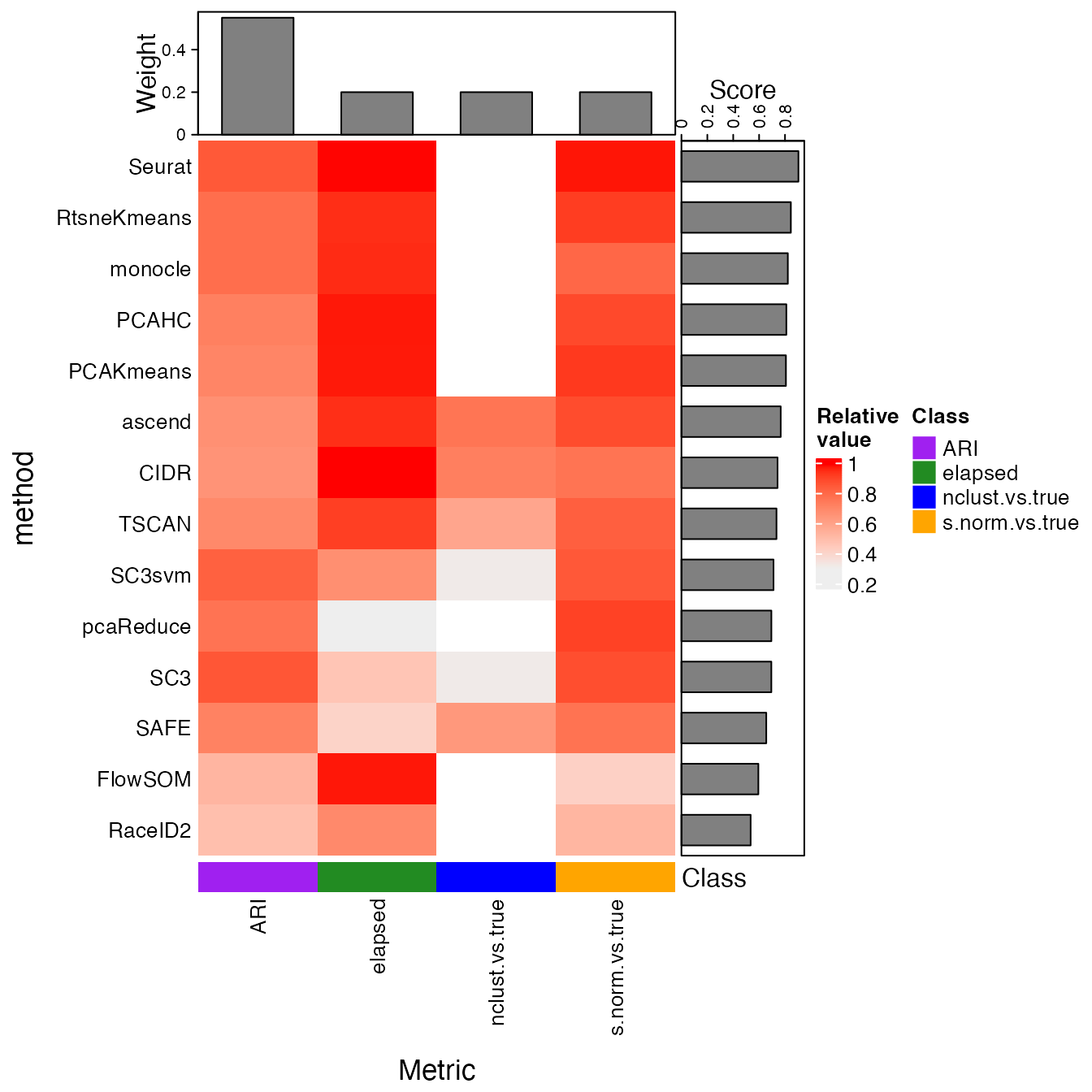
makePolarPlot(bettrList = prepData)
#> Warning: Removed 8 rows containing missing values or values outside the scale range
#> (`geom_col()`).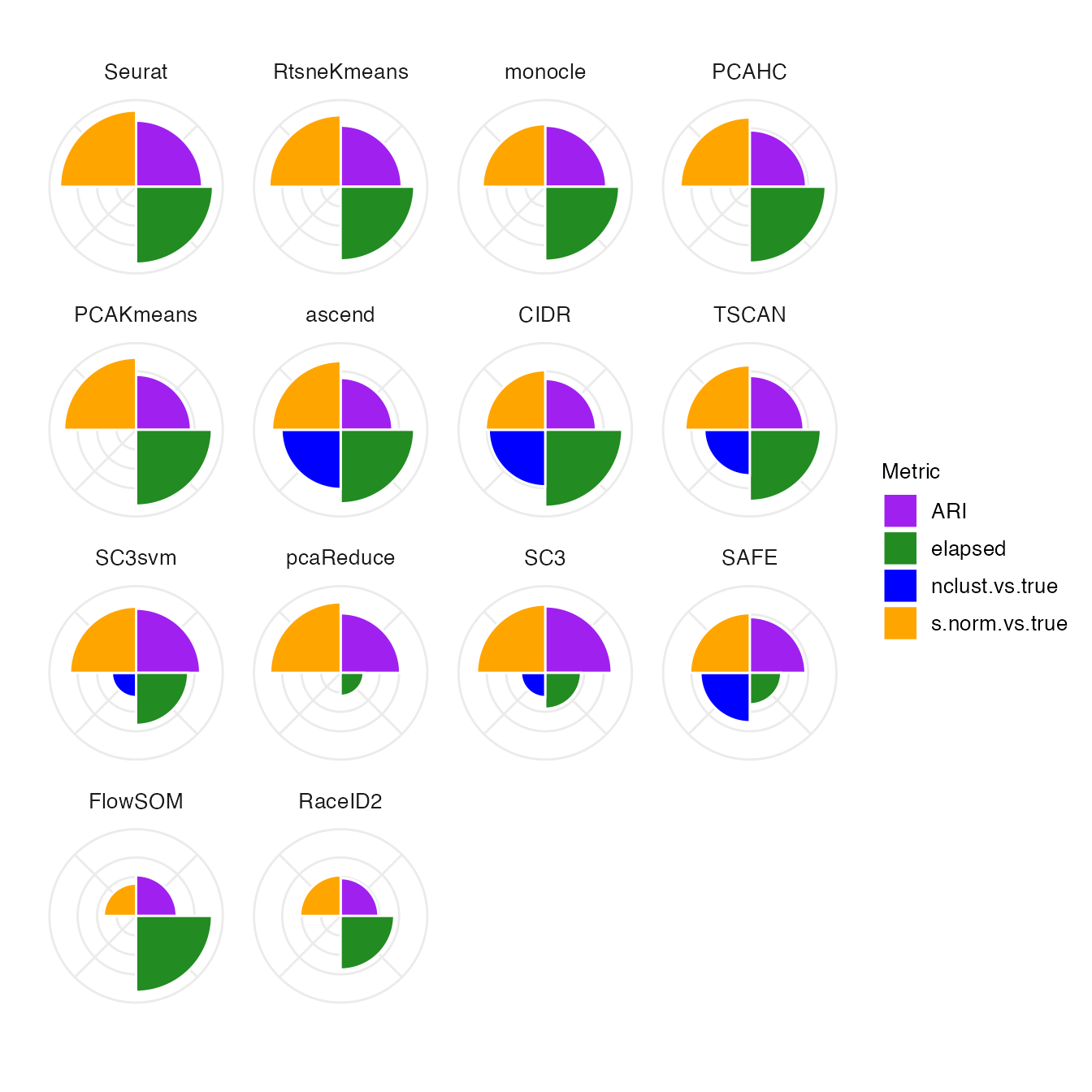
Exporting data from the app
It is possible to export the data used internally by the interactive
application, in the same format as the output from
bettrGetReady(). To enable such export, first generate the
app object using the bettr() function, and
then assign the call to shiny::runApp() to a variable to
capture the output. For example:
if (interactive()) {
    app <- bettr(bettrSE = duo2018, bstheme = "sandstone")
    out <- shiny::runApp(app)
}
To activate the export, make sure to click the button ‘Close app’ (in
the bottom of the left-hand side bar) in order to close the application
(don’t just close the window). This will take you back to your R
session, where the variable out will be populated with the
data used in the app (in the same format as the output from
bettrGetReady()). This list can be directly provided as the
input to e.g. makeHeatmap() and the other plotting
functions via the bettrList argument, as shown above.
Additional examples
bettr can also be adapted to represent other types of
collections of metric scores than the results of benchmarking studies in
computational biology. An example,
which is also included in the inst/scripts folder of this
package, presents the OECD Better Life Index (https://stats.oecd.org/index.aspx?DataSetCode=BLI),
spanning over 11 topics, each represented by one to three indicators.
These indicators are measures of the concepts of well-being, and well
suited to display some comparison across countries.
Additional examples can be added to the codebase upon interest, and we encourage users to contribute to that via a Pull Request to https://github.com/federicomarini/bettr.
Session info
sessionInfo()
#> R version 4.6.0 Patched (2026-04-27 r89967)
#> Platform: aarch64-apple-darwin23
#> Running under: macOS Sequoia 15.7.4
#>
#> Matrix products: default
#> BLAS:   /Library/Frameworks/R.framework/Versions/4.6/Resources/lib/libRblas.0.dylib
#> LAPACK: /Library/Frameworks/R.framework/Versions/4.6/Resources/lib/libRlapack.dylib;  LAPACK version 3.12.1
#>
#> locale:
#> [1] en_US.UTF-8/en_US.UTF-8/en_US.UTF-8/C/en_US.UTF-8/en_US.UTF-8
#>
#> time zone: UTC
#> tzcode source: internal
#>
#> attached base packages:
#> [1] stats4    stats     graphics  grDevices utils     datasets  methods
#> [8] base
#>
#> other attached packages:
#>  [1] dplyr_1.2.1                 tibble_3.3.1
#>  [3] SummarizedExperiment_1.41.1 Biobase_2.71.0
#>  [5] GenomicRanges_1.63.2        Seqinfo_1.1.0
#>  [7] IRanges_2.45.0              S4Vectors_0.49.2
#>  [9] BiocGenerics_0.57.1         generics_0.1.4
#> [11] MatrixGenerics_1.23.0       matrixStats_1.5.0
#> [13] bettr_1.9.0                 BiocStyle_2.39.0
#>
#> loaded via a namespace (and not attached):
#>  [1] gridExtra_2.3         rlang_1.2.0           magrittr_2.0.5
#>  [4] clue_0.3-68           GetoptLong_1.1.1      otel_0.2.0
#>  [7] compiler_4.6.0        png_0.1-9             systemfonts_1.3.2
#> [10] vctrs_0.7.3           stringr_1.6.0         pkgconfig_2.0.3
#> [13] shape_1.4.6.1         crayon_1.5.3          fastmap_1.2.0
#> [16] backports_1.5.1       XVector_0.51.0        labeling_0.4.3
#> [19] utf8_1.2.6            learnr_0.11.6         shinyjqui_0.4.1
#> [22] promises_1.5.0        rmarkdown_2.31        ragg_1.5.2
#> [25] purrr_1.2.2           xfun_0.57             cachem_1.1.0
#> [28] jsonlite_2.0.0        later_1.4.8           DelayedArray_0.37.1
#> [31] parallel_4.6.0        cluster_2.1.8.2       R6_2.6.1
#> [34] bslib_0.10.0          stringi_1.8.7         RColorBrewer_1.1-3
#> [37] rpart_4.1.27          jquerylib_0.1.4       assertthat_0.2.1
#> [40] Rcpp_1.1.1-1.1        bookdown_0.46         iterators_1.0.14
#> [43] knitr_1.51            base64enc_0.1-6       httpuv_1.6.17
#> [46] Matrix_1.7-5          nnet_7.3-20           tidyselect_1.2.1
#> [49] rstudioapi_0.18.0     abind_1.4-8           yaml_2.3.12
#> [52] doParallel_1.0.17     codetools_0.2-20      lattice_0.22-9
#> [55] withr_3.0.2           shiny_1.13.0          S7_0.2.2
#> [58] evaluate_1.0.5        foreign_0.8-91        desc_1.4.3
#> [61] circlize_0.4.18       pillar_1.11.1         BiocManager_1.30.27
#> [64] checkmate_2.3.4       DT_0.34.0             foreach_1.5.2
#> [67] rprojroot_2.1.1       ggplot2_4.0.3         scales_1.4.0
#> [70] xtable_1.8-8          glue_1.8.1            Hmisc_5.2-5
#> [73] tools_4.6.0           data.table_1.18.2.1   fs_2.1.0
#> [76] cowplot_1.2.0         grid_4.6.0            tidyr_1.3.2
#> [79] sortable_0.6.0        colorspace_2.1-2      htmlTable_2.5.0
#> [82] Formula_1.2-5         cli_3.6.6             textshaping_1.0.5
#> [85] S4Arrays_1.11.1       ComplexHeatmap_2.27.1 gtable_0.3.6
#> [88] sass_0.4.10           digest_0.6.39         SparseArray_1.11.13
#> [91] rjson_0.2.23          htmlwidgets_1.6.4     farver_2.1.2
#> [94] htmltools_0.5.9       pkgdown_2.2.0.9000    lifecycle_1.0.5
#> [97] GlobalOptions_0.1.4   mime_0.13