GeneTonic: enjoying the interpretation of your RNA-seq data analysis
Federico Marini
Institute of Medical Biostatistics, Epidemiology and Informatics (IMBEI), MainzCenter for Thrombosis and Hemostasis (CTH), Mainzmarinif@uni-mainz.de
Annekathrin Ludt
Institute of Medical Biostatistics, Epidemiology and Informatics (IMBEI), Mainzanneludt@uni-mainz.de Source:
vignettes/GeneTonicWorkshop.Rmd
GeneTonicWorkshop.RmdSetup for this workshop
To install the GeneTonic package and the package for this workshop, containing a processed version of the example dataset, execute the following chunk:
# from Bioconductor
BiocManager::install("GeneTonic")
# devel version on GitHub
BiocManager::install("federicomarini/GeneTonic")
# this workshop
BiocManager::install("federicomarini/GeneTonicWorkshop",
                     build_vignettes = TRUE,
                     dependencies = TRUE)
That should be it!
To make sure everything is installed correctly, run
Using GeneTonic on the A20-deficient microglia dataset (GSE123033)
About the data
The data illustrated in this document is an RNA-seq dataset, available at the GEO repository under the accession code GSE123033 (https://www.ncbi.nlm.nih.gov/geo/query/acc.cgi?acc=GSE123033).
This was generated as a part of the work to elucidate the role of microglial A20 in maintaining brain homeostasis, comparing fully deficient to partially deficient microglia tissue (Mohebiany et al. 2020) - the manuscript is available at https://www.sciencedirect.com/science/article/pii/S2211124719317620.
Loading required packages
We load the packages required to perform all the analytic steps presented in this document.
Data processing - Exploratory data analysis
After obtaining a count matrix (via STAR and featureCounts), we generated a DESeqDataset object, provided in this repository for the ease of reproducing the presented analyses.
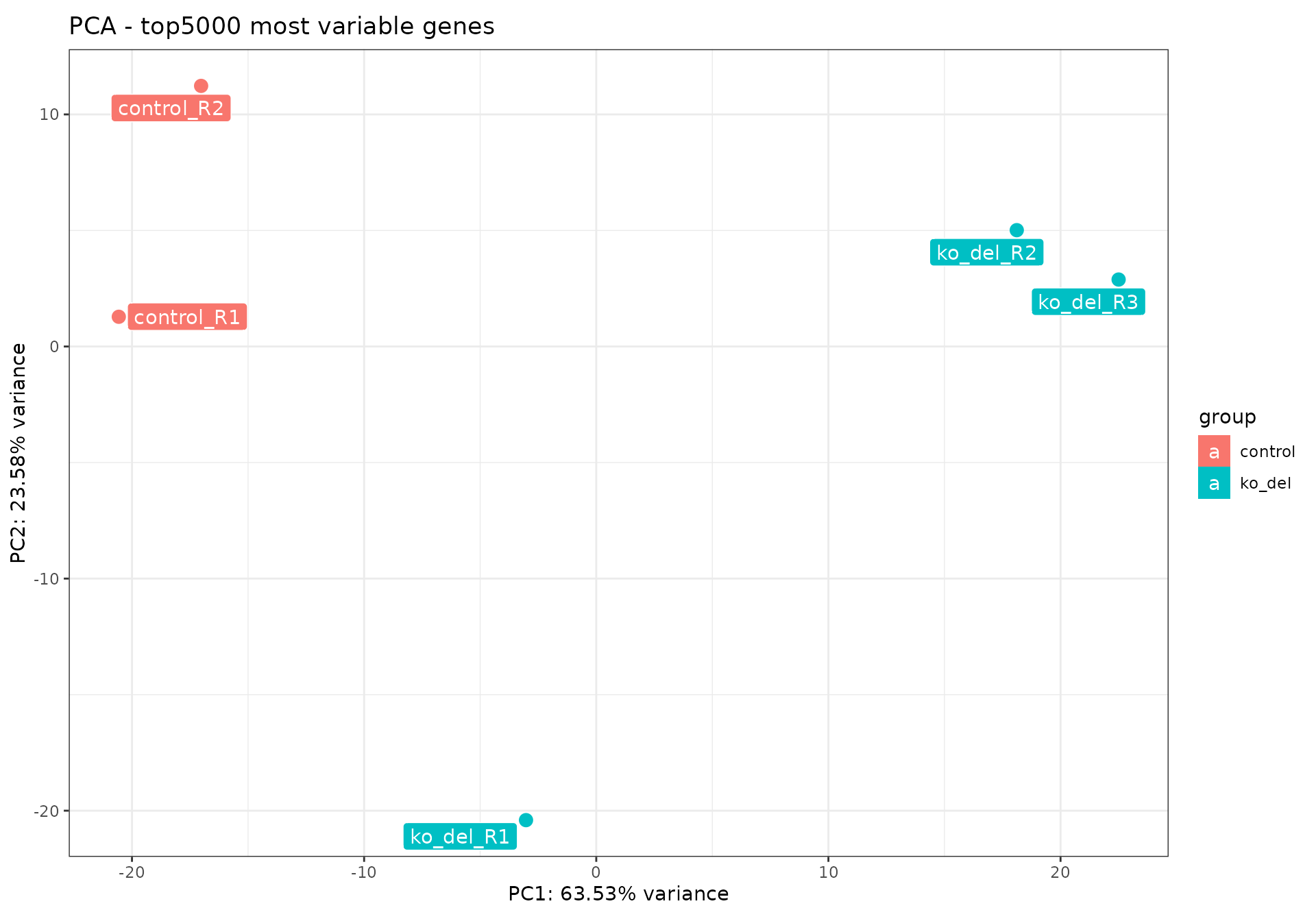
We read in the dataset, apply the rlog transformation for performing PCA and creating a heatmap of the sample to sample distances.
We’ll use some functions from the pcaExplorer package (Marini and Binder 2019) (see also Supplementary Figure 3 of (Mohebiany et al. 2020)).
These are the preprocessed dataset we are going to use throughout the demo:
list.files(system.file("extdata", package = "GeneTonicWorkshop"))
#> [1] "gtl_alma.rds"                "usecase_annodf_alma.rds"
#> [3] "usecase_dds_alma.rds"        "usecase_res_de_alma.rds"
#> [5] "usecase_res_enrich_alma.rds"
We load the DESeqDataSet object and the annotation data frame for handling the conversion between Ensembl ids and gene names, and do a quick exploration of the data
dds_alma <- readRDS(
  system.file("extdata", "usecase_dds_alma.rds", package = "GeneTonicWorkshop")
)
dds_alma
#> class: DESeqDataSet
#> dim: 41388 5
#> metadata(1): version
#> assays(4): counts mu H cooks
#> rownames(41388): ENSMUSG00000090025 ENSMUSG00000064842 ...
#>   ENSMUSG00000096730 ENSMUSG00000095742
#> rowData names(22): baseMean baseVar ... deviance maxCooks
#> colnames(5): control_R1 control_R2 ko_del_R1 ko_del_R2 ko_del_R3
#> colData names(8): fastqfile bamfile ... sampleName sizeFactor

rld_alma <- rlogTransformation(dds_alma)

anno_df <- readRDS(
  system.file("extdata", "usecase_annodf_alma.rds", package = "GeneTonicWorkshop")
)

pheatmap::pheatmap(as.matrix(dist(t(assay(rld_alma)))))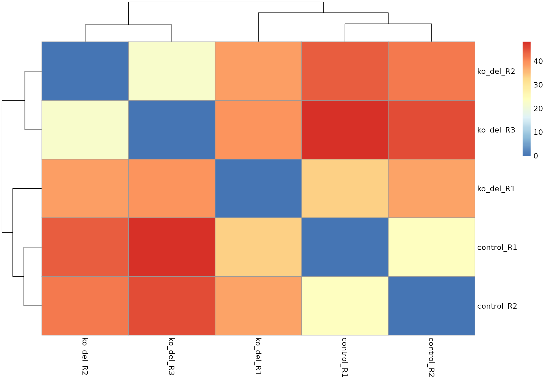
pcaExplorer::pcaplot(rld_alma,
  ntop = 5000,
  title = "PCA - top5000 most variable genes",
  ellipse = FALSE
)
Data processing - Differential expression analysis
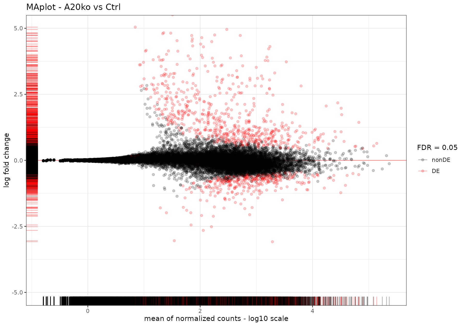
We set the False Discovery Rate to 0.05 and we run the DESeq2 workflow, generating results and using the apeglm shrinkage estimator.
We plot the results as an MA-plot and report them in a table, using the functions from the ideal package (Marini, Linke, and Binder 2020) (see also Supplementary Figure 3 of (Mohebiany et al. 2020)).
FDR <- 0.05

dds_alma <- DESeq(dds_alma)

res_alma_ko_vs_ctrl <- results(dds_alma, name = "condition_ko_del_vs_control", alpha = FDR)
summary(res_alma_ko_vs_ctrl)
#>
#> out of 20699 with nonzero total read count
#> adjusted p-value < 0.05
#> LFC > 0 (up)       : 668, 3.2%
#> LFC < 0 (down)     : 342, 1.7%
#> outliers [1]       : 3, 0.014%
#> low counts [2]     : 7984, 39%
#> (mean count < 5)
#> [1] see 'cooksCutoff' argument of ?results
#> [2] see 'independentFiltering' argument of ?results
library("apeglm")
res_alma_ko_vs_ctrl <- lfcShrink(dds_alma, coef = "condition_ko_del_vs_control", type = "apeglm", res = res_alma_ko_vs_ctrl)

res_alma_ko_vs_ctrl$SYMBOL <- anno_df$gene_name[match(rownames(res_alma_ko_vs_ctrl), anno_df$gene_id)]

summary(res_alma_ko_vs_ctrl)
#>
#> out of 20699 with nonzero total read count
#> adjusted p-value < 0.05
#> LFC > 0 (up)       : 668, 3.2%
#> LFC < 0 (down)     : 342, 1.7%
#> outliers [1]       : 3, 0.014%
#> low counts [2]     : 7984, 39%
#> (mean count < 5)
#> [1] see 'cooksCutoff' argument of ?results
#> [2] see 'independentFiltering' argument of ?results

# saveRDS(res_alma_ko_vs_ctrl, file = "../inst/extdata/usecase_res_de_alma.rds")
Alternatively, we load in the results from the object included in the package
res_alma_ko_vs_ctrl <- readRDS(
  system.file("extdata", "usecase_res_de_alma.rds", package = "GeneTonicWorkshop")
)
tbl_DEres_alma_ko_vs_ctrl <- GeneTonic::deseqresult2df(res_alma_ko_vs_ctrl, FDR = FDR)

DT::datatable(tbl_DEres_alma_ko_vs_ctrl, rownames = FALSE)
Data processing - Functional enrichment analysis
We perform functional enrichment analysis, here using the topGOtable wrapper (from pcaExplorer) to the method implemented in the topGO package.
expressedInAssay <- (rowSums(assay(dds_alma)) > 0)
geneUniverseExprENS <- rownames(dds_alma)[expressedInAssay]
geneUniverseExpr <- anno_df$gene_name[match(geneUniverseExprENS, anno_df$gene_id)]

GObps_ko_vs_ctrl <- topGOtable(
  DEgenes = tbl_DEres_alma_ko_vs_ctrl$SYMBOL,
  BGgenes = geneUniverseExpr,
  ontology = "BP",
  geneID = "symbol",
  addGeneToTerms = TRUE,
  mapping = "org.Mm.eg.db",
  topTablerows = 500
)

GOmfs_ko_vs_ctrl <- topGOtable(
  DEgenes = tbl_DEres_alma_ko_vs_ctrl$SYMBOL,
  BGgenes = geneUniverseExpr,
  ontology = "MF",
  geneID = "symbol",
  addGeneToTerms = TRUE,
  mapping = "org.Mm.eg.db",
  topTablerows = 500
)

GOccs_ko_vs_ctrl <- topGOtable(
  DEgenes = tbl_DEres_alma_ko_vs_ctrl$SYMBOL,
  BGgenes = geneUniverseExpr,
  ontology = "CC",
  geneID = "symbol",
  addGeneToTerms = TRUE,
  mapping = "org.Mm.eg.db",
  topTablerows = 500
)
We take for example the results of the enrichment in the Biological Processes ontology, and convert them for use in GeneTonic
res_enrich_a20 <- shake_topGOtableResult(GObps_ko_vs_ctrl)We compute some aggregated scores - this additional columns will come in handy to colorize points, encoding for information about the direction of regulation of each biological process
res_enrich_a20 <- get_aggrscores(
  res_enrich = res_enrich_a20,
  res_de = res_alma_ko_vs_ctrl,
  annotation_obj = anno_df
)

# saveRDS(res_enrich_a20, file = "../inst/extdata/usecase_res_enrich_alma.rds")

DT::datatable(res_enrich_a20, rownames = FALSE)
If desired, you can load directly the enrichment results, already converted for GeneTonic, from the objects provided in this workshop package:
res_enrich_a20 <- readRDS(
  system.file("extdata", "usecase_res_enrich_alma.rds", package = "GeneTonicWorkshop")
)
Using alternative enrichment analysis methods
It is possible to use the output of different other methods for enrichment analysis, thanks to the shaker_* functions implemented in GeneTonic - see for example ?shake_topGOtableResult, and navigate to the manual pages for the other functions listed in the “See Also” section.
GeneTonic is able to convert for you the output of
- DAVID (text file, downloaded from the DAVID website)
- clusterProfiler (takes
enrichResultobjects) - enrichr (a data.frame with the output of
enrichr, or the text file exported from Enrichr) - fgsea (the output of
fgsea()function) - g:Profiler (the text file output as exported from g:Profiler, or a data.frame with the output of
gost()ingprofiler2)
Some examples on how to use them are reported here:
# clusterProfiler --------------------------------------------------------------
library("clusterProfiler")
degenes_alma <- deseqresult2df(res_alma_ko_vs_ctrl, FDR = 0.05)$id
ego_alma <- enrichGO(
  gene = degenes_alma,
  universe = rownames(dds_alma)[expressedInAssay],
  OrgDb = org.Mm.eg.db,
  ont = "BP",
  keyType = "ENSEMBL",
  pAdjustMethod = "BH",
  pvalueCutoff = 0.01,
  qvalueCutoff = 0.05,
  readable = TRUE
)
res_enrich_clusterprofiler <- shake_enrichResult(ego_alma)

# g:profiler -------------------------------------------------------------------
library("gprofiler2")
degenes <- deseqresult2df(res_alma_ko_vs_ctrl, FDR = 0.05)$SYMBOL
gostres_a20 <- gost(
  query = degenes,
  ordered_query = FALSE,
  multi_query = FALSE,
  significant = FALSE,
  exclude_iea = TRUE,
  measure_underrepresentation = FALSE,
  evcodes = TRUE,
  user_threshold = 0.05,
  correction_method = "g_SCS",
  domain_scope = "annotated",
  numeric_ns = "",
  sources = "GO:BP",
  as_short_link = FALSE
)

res_enrich_gprofiler <- shake_gprofilerResult(gprofiler_output = gostres_a20$result)

# fgsea ------------------------------------------------------------------------
library("dplyr")
library("tibble")
library("fgsea")
library("msigdbr")
res2 <- res_alma_ko_vs_ctrl %>%
  as.data.frame() %>%
  dplyr::select(SYMBOL, log2FoldChange)
de_ranks <- deframe(res2)
msigdbr_df <- msigdbr(species = "Mus musculus", category = "C5", subcategory = "BP")
msigdbr_list <- split(x = msigdbr_df$gene_symbol, f = msigdbr_df$gs_name)
fgseaRes <- fgsea(
  pathways = msigdbr_list,
  stats = de_ranks,
  nperm = 100000
)
fgseaRes <- fgseaRes %>%
  arrange(desc(NES))

res_enrich_fgsea <- shake_fgseaResult(fgsea_output = fgseaRes)

# enrichr ----------------------------------------------------------------------
library("enrichR")
dbs <- c(
  "GO_Molecular_Function_2018",
  "GO_Cellular_Component_2018",
  "GO_Biological_Process_2018",
  "KEGG_2019_Human",
  "Reactome_2016",
  "WikiPathways_2019_Human"
)
degenes <- (deseqresult2df(res_alma_ko_vs_ctrl, FDR = 0.05)$SYMBOL)
enrichr_output_a20 <- enrichr(degenes, dbs)

res_enrich_enrichr_BPs <- shake_enrichrResult(
  enrichr_output = enrichr_output_a20$GO_Biological_Process_2018
)
res_enrich_enrichr_KEGG <- shake_enrichrResult(
  enrichr_output = enrichr_output_a20$KEGG_2019_Human
)
Assembling the gtl object
To simplify the usage of the function from GeneTonic, we create a GeneTonic_list object
gtl_alma <- GeneTonic_list(
  dds = dds_alma,
  res_de = res_alma_ko_vs_ctrl,
  res_enrich = res_enrich_a20,
  annotation_obj = anno_df
)

# saveRDS(gtl_alma, "../inst/extdata/gtl_alma.rds")
Again, if desired, you could load the gtl object directly from the precomputed objects
gtl_alma <- readRDS(
  system.file("extdata", "gtl_alma.rds", package = "GeneTonicWorkshop")
)
Running GeneTonic on the dataset, interactively
We do have a GeneTonicList object, containing all the structured input needed.
We can inspect its content with the internal GeneTonic:::describe_gtl()
GeneTonic:::describe_gtl(gtl_alma)This command will launch the GeneTonic app:
GeneTonic(gtl = gtl_alma)The exploration can be guided by launching the introductory tours for each section of the app, and finally one can generate a small report focused on the features and genesets of interest.
Exploring the GeneTonic app
The GeneTonic app provides various different panels and plots to visualize your data. When launching the app as shown above, the GeneTonic app will start and show information about the provided data in the Welcome panel.
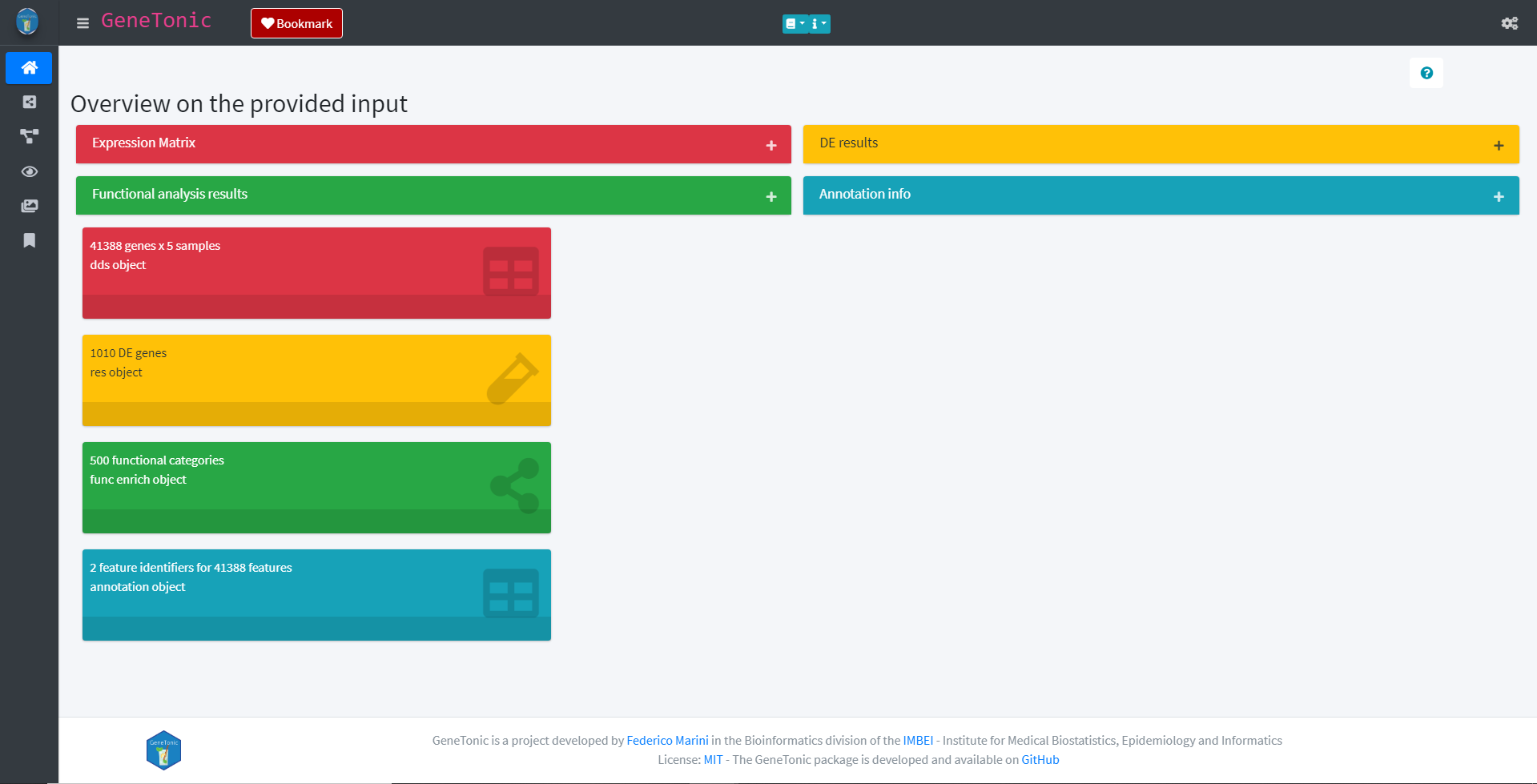
GeneTonic Welcome panel
The panel list the individual inputs of the GeneTonic app with some overall information (e.g. the number of DE genes). Further information about the input can be acquired by clicking the plus sign of each respective input.
Via the panel selection on the left side, individual panels can be explored. One of these panels is the Gene-Geneset panel which provides information about the genesets and genes found in the data based on the functional annotation object. The genesets and their belonging genes are depicted in a graph in which the genesets are shown as yellow rectangles and the genes as round nodes. The node color of the genes reflects their regulation in the data with red indicating an up-regulation and blue a down-regulation.
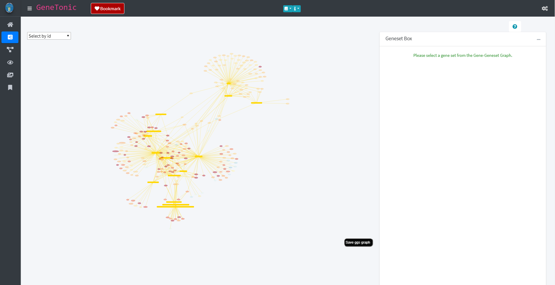
Gene-Geneset panel
Each panel offers a variety of different possibilities and options to explore the data. In order to familiarize with these options, each panel has a guided tour which highlights and explains the different possibilities. The tour can be started by clicking on the question mark button (in the image above this the button can be found above the Geneset box). The button activates the tour which will open as a small window on the screen.
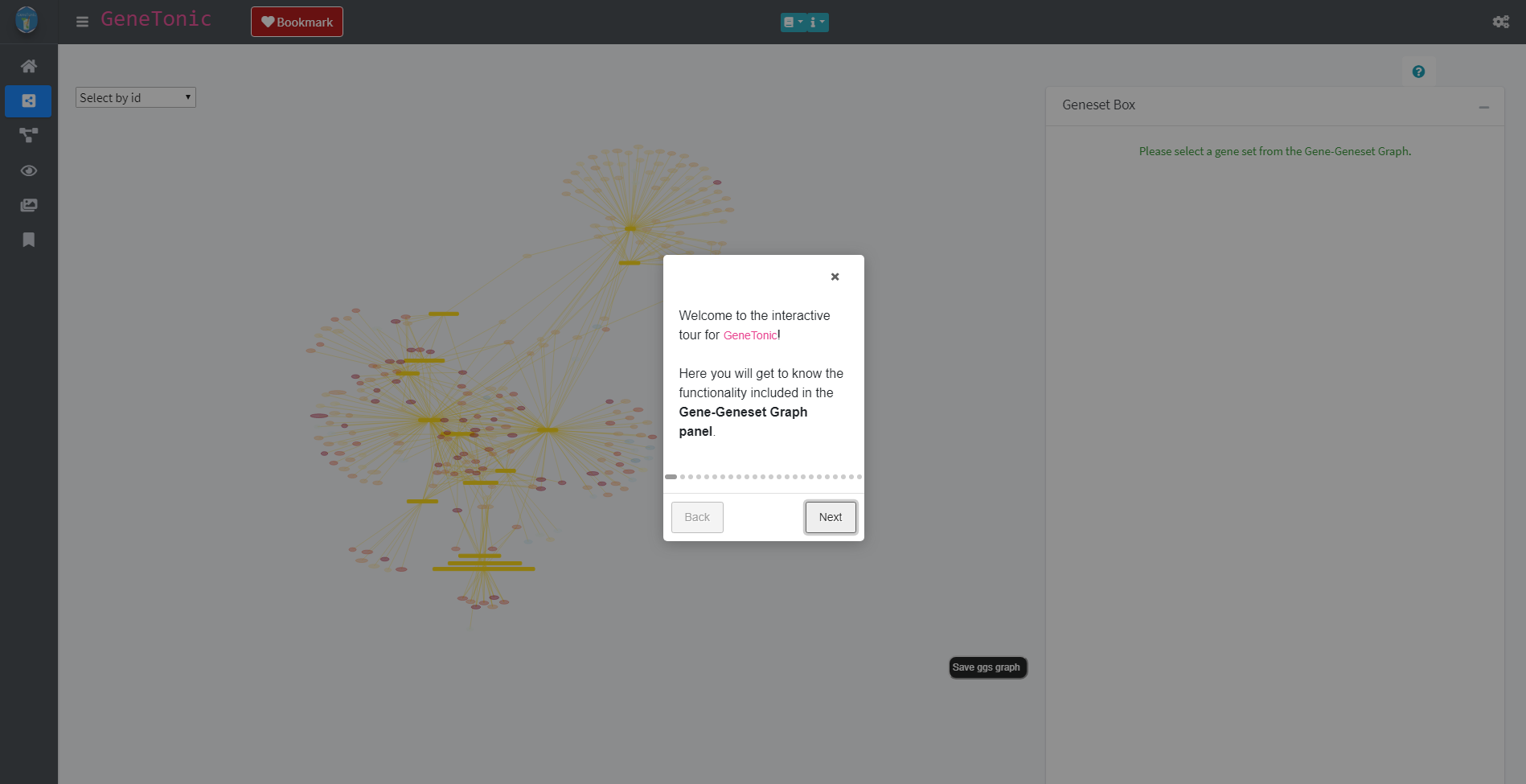
Start of the tour
The “Next” and “Back” button lead through the tour and its individual elements. Throughout the tour individual elements of the respective panel will be highlighted and explained.
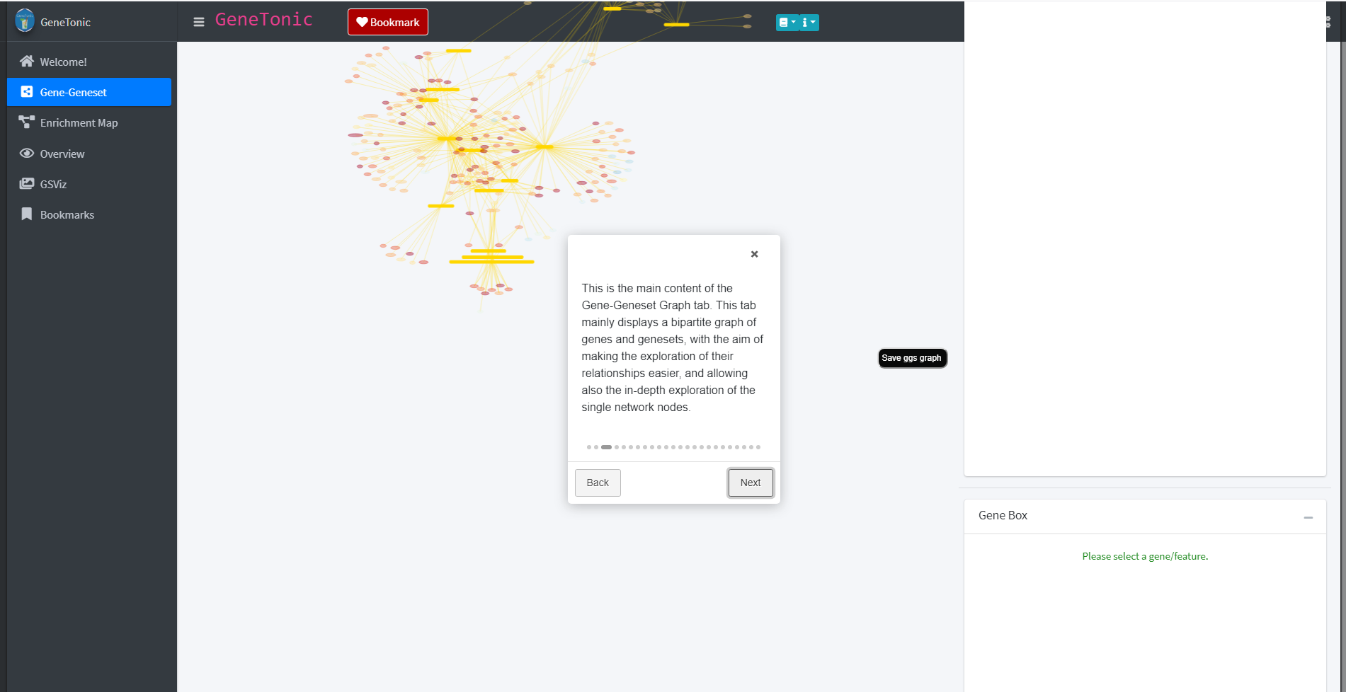 The panels of the
 GeneTonic app are designed interactively and offer the possibility of exploring the data by clicking on various elements of the page. For example through clicking on one of the genesets in the shown graph (yellow rectangle) additional content will be displayed in the Geneset box. In the case of a geneset these are a heatmap and a volcano plot which provide additional information about the regulation of the genes contained in the geneset.
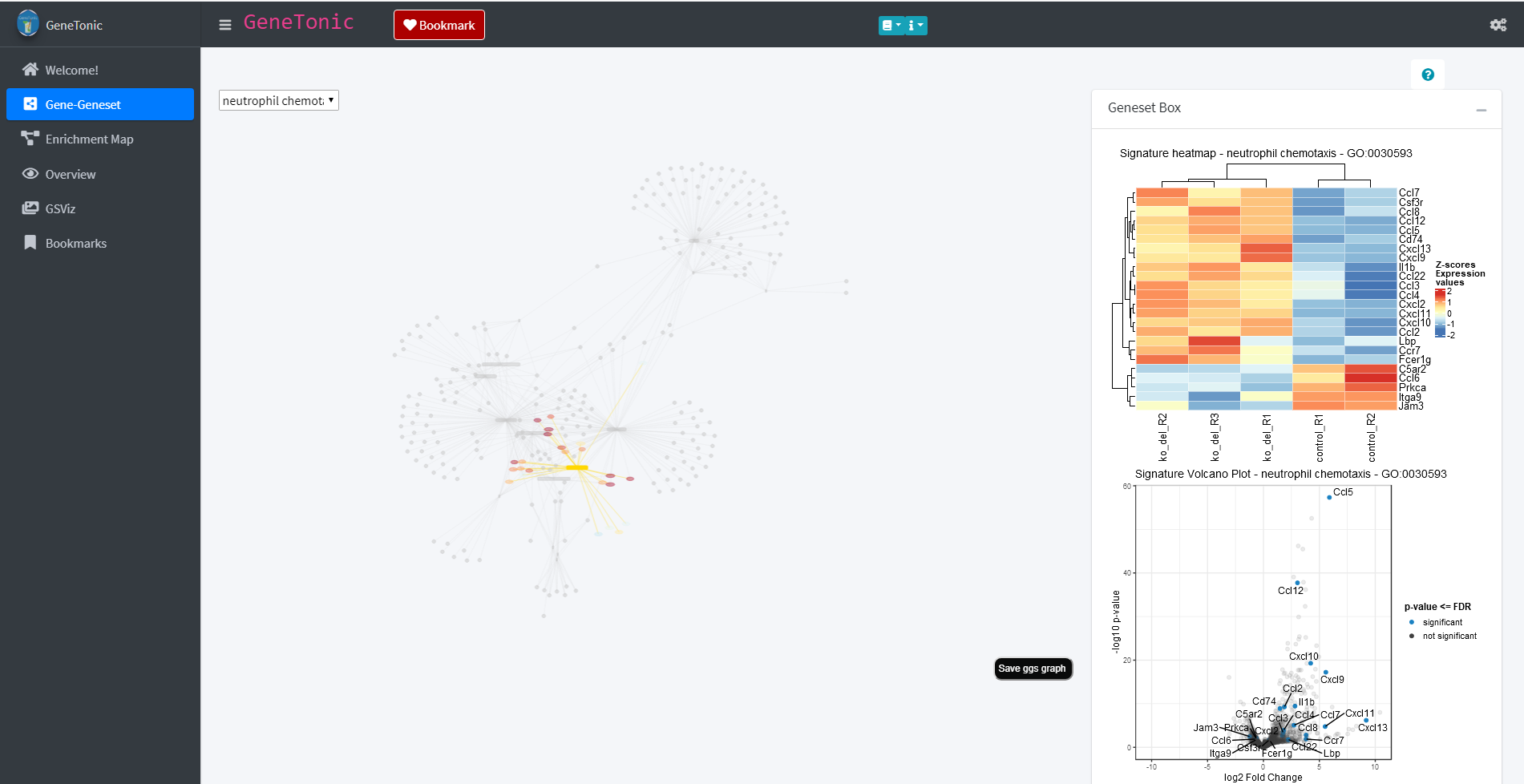
Geneset Box
The information provided by the heatmap and volcano plot of each geneset can further be broadened. For this several options are provided through clicking on the cog-wheel symbol in the upper right corner of the page. This opens a sidebar with several additional options. These options include the choice of FDR threshold, the number of genesets displayed in the main graph of the page or a drop-down menu which allows to group/color the displayed heatmap by different factors e.g. the sample id.
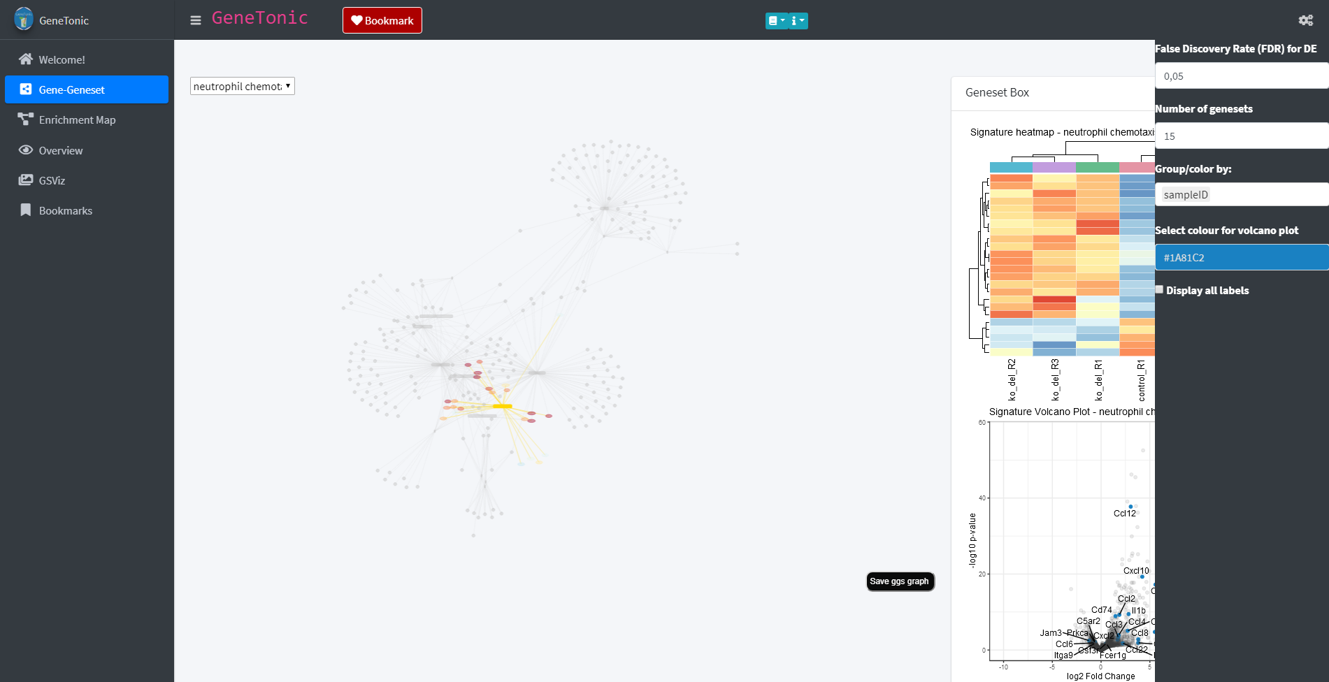
Different additional possibilities are offered through a sidebar menu
GeneTonic offers a wide range of visualizations of the data in each of the individual panels ranging from birds-eye view plots to detailed plots about specific subsets of the data. However, if some more custom visualizations are required, it is possible to export the objects in use from the app as a SummarizedExperiment object, to be then passed to the iSEE software (Rue-Albrecht et al. 2018) for further exploration.
Furthermore, the app also offers the possibility to generate a report about genes and genesets of interest. This can be achieved by bookmarking those genes and genesets via the “Bookmark” button found in each panel. The report and SummarizedExperiment object can then be generated in the Bookmark panel by clicking the button “Start the happy hour!” (for the report) or “Export as serialized SummarizedExperiment” (for the SummarizedExperiment)
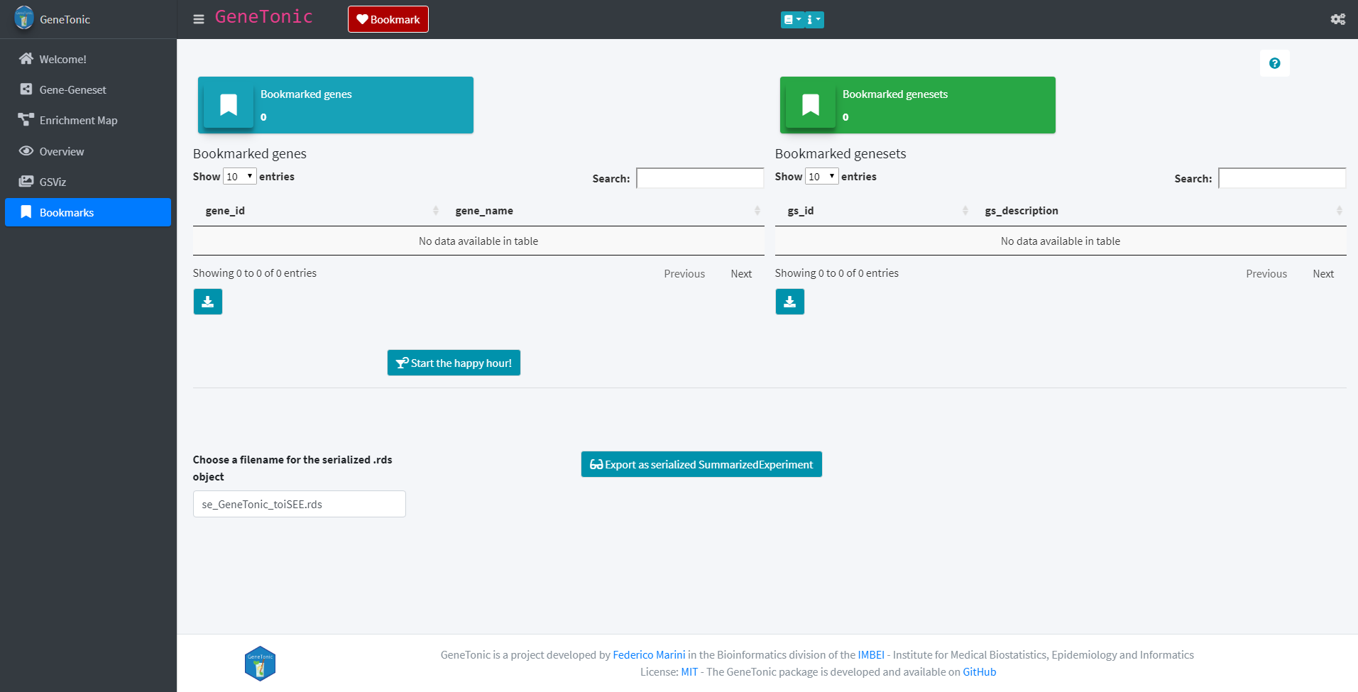
Exporting the data for further use
Using GeneTonic’s functions in analysis reports
The functionality of GeneTonic can be used also as standalone functions, to be called for example in existing analysis reports in RMarkdown, or R scripts.
In the following chunks, we show how it is possible to call some of the functions on the A20-deficient microglia set.
For more details on the functions and their outputs, please refer to the package documentation and the vignette.
Genesets and genes
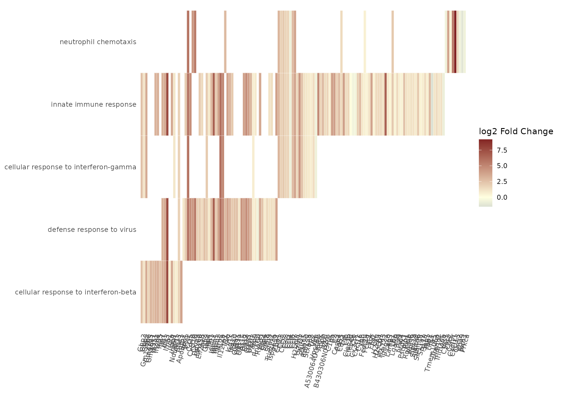
We can represent the relationships between genesets and genes with enhance_table(), gs_summary_heat(), and ggs_graph():
p <- enhance_table(
  gtl = gtl_alma,
  n_gs = 30,
  chars_limit = 60
)
p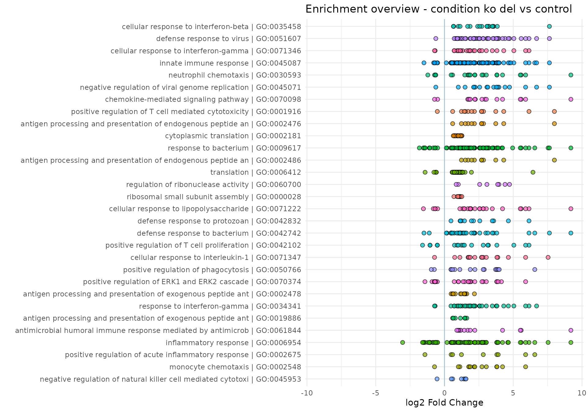
## could be made interactive with...
# library("plotly")
# ggplotly(p)

gs_summary_heat(
  gtl = gtl_alma,
  n_gs = 5
)
ggs <- ggs_graph(
gtl = gtl_alma,
n_gs = 20
)
ggs
#> IGRAPH edf83c9 UN-- 291 626 --
#> + attr: name (v/c), nodetype (v/c), shape (v/c), color (v/c), title
#> | (v/c)
#> + edges from edf83c9 (vertex names):
#> [1] cellular response to interferon-beta--Gbp2
#> [2] cellular response to interferon-beta--Gbp3
#> [3] cellular response to interferon-beta--Gbp6
#> [4] cellular response to interferon-beta--Gm12185
#> [5] cellular response to interferon-beta--Gm4841
#> [6] cellular response to interferon-beta--Gm4951
#> [7] cellular response to interferon-beta--Ifi204
#> + ... omitted several edges
## could be viewed interactively with
library("visNetwork")
library("magrittr")
ggs %>%
visIgraph() %>%
visOptions(
highlightNearest = list(
enabled = TRUE,
degree = 1,
hover = TRUE
),
nodesIdSelection = TRUE
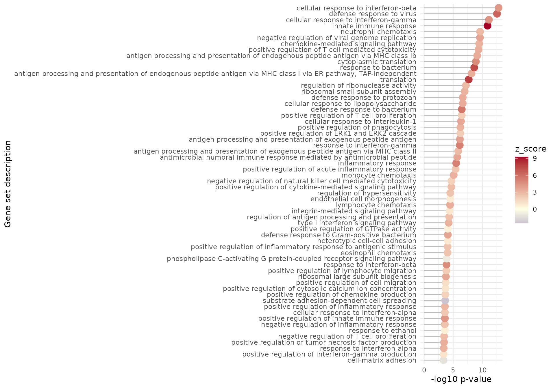
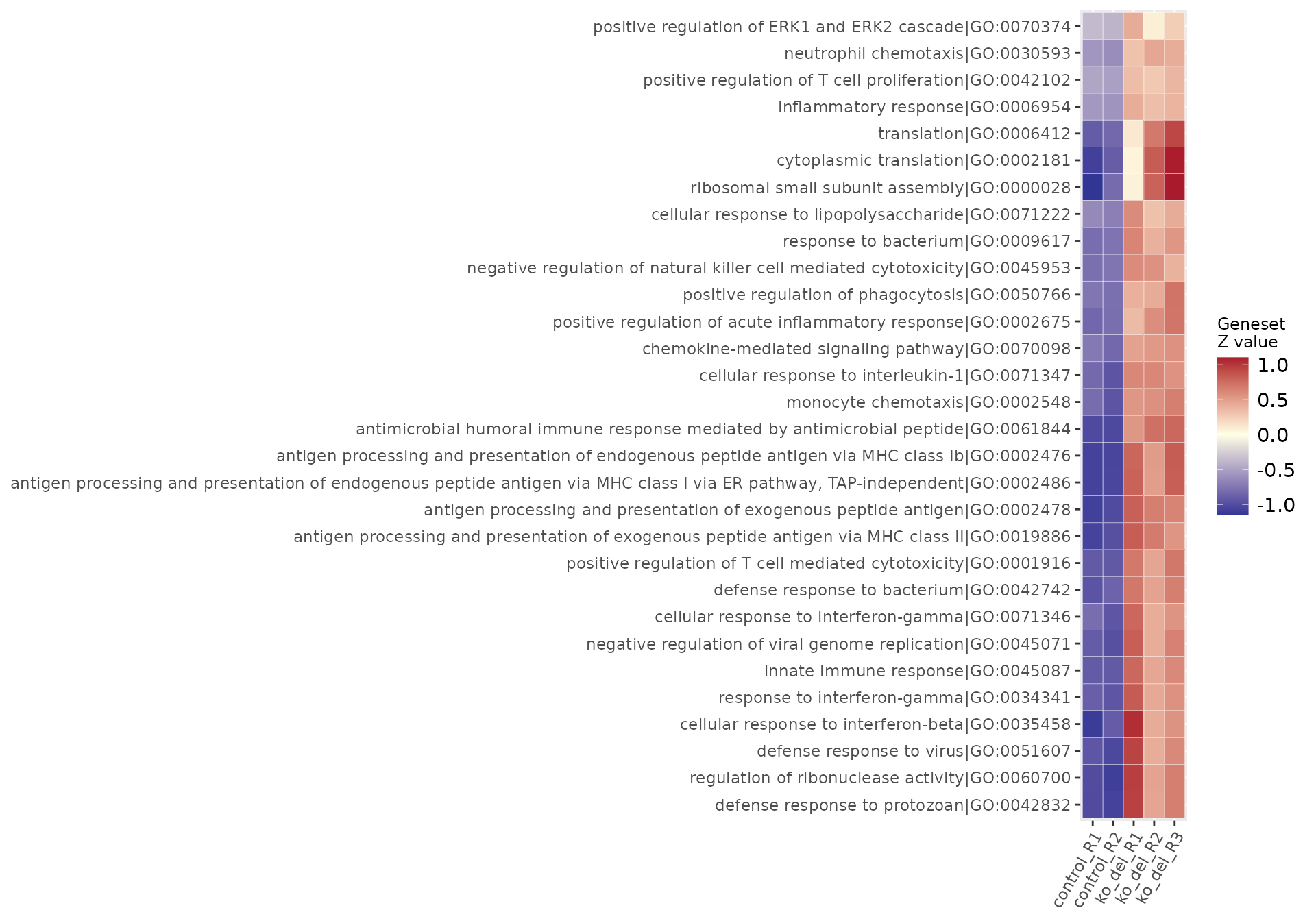
)Overview representations
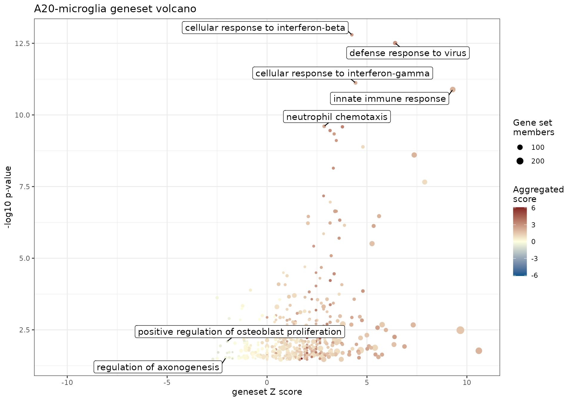
We can also obtain summary representations of the enrichment results, either as table-like views (with gs_volcano(), gs_summary_overview(), gs_fuzzyclustering(), gs_scoresheat()), or to represent the relationships among genesets (via enrichment_map(), gs_dendro(), gs_mds())
gs_volcano(
  res_enrich = res_enrich_a20,
  p_threshold = 0.05,
  color_by = "aggr_score",
  volcano_labels = 5,
  gs_ids = c("GO:0033690", "GO:0050770"),
  plot_title = "A20-microglia geneset volcano"
)
gs_summary_overview(
  res_enrich = res_enrich_a20,
  n_gs = 60,
  p_value_column = "gs_pvalue",
  color_by = "z_score"
)
res_enrich_subset <- res_enrich_a20[1:200, ]
fuzzy_subset <- gs_fuzzyclustering(
  res_enrich = res_enrich_subset,
  n_gs = nrow(res_enrich_subset),
  gs_ids = NULL,
  similarity_matrix = NULL,
  similarity_threshold = 0.35,
  fuzzy_seeding_initial_neighbors = 3,
  fuzzy_multilinkage_rule = 0.5
)

# show all genesets members of the first cluster
DT::datatable(
  fuzzy_subset[fuzzy_subset$gs_fuzzycluster == "1", ]
)
em <- enrichment_map(gtl = gtl_alma, n_gs = 100)

library("visNetwork")
library("magrittr")
em %>%
  visIgraph() %>%
  visOptions(
    highlightNearest = list(
      enabled = TRUE,
      degree = 1,
      hover = TRUE
    ),
    nodesIdSelection = TRUE
  )

distilled <- distill_enrichment(
  gtl = gtl_alma,
  n_gs = 100,
  cluster_fun = "cluster_markov"
)
DT::datatable(distilled$distilled_table)
DT::datatable(distilled$res_enrich)

dg <- distilled$distilled_em

library("igraph")
library("visNetwork")
library("magrittr")

# defining a color palette for nicer display
colpal <- colorspace::rainbow_hcl(length(unique(V(dg)$color)))[V(dg)$color]
V(dg)$color.background <- scales::alpha(colpal, alpha = 0.8)
V(dg)$color.highlight <- scales::alpha(colpal, alpha = 1)
V(dg)$color.hover <- scales::alpha(colpal, alpha = 0.5)

V(dg)$color.border <- "black"

visNetwork::visIgraph(dg) %>%
  visOptions(
    highlightNearest = list(
      enabled = TRUE,
      degree = 1,
      hover = TRUE
    ),
    nodesIdSelection = TRUE,
    selectedBy = "membership"
  )


gs_dendro(
  gtl = gtl_alma,
  n_gs = 50,
  gs_dist_type = "kappa",
  clust_method = "ward.D2",
  color_leaves_by = "z_score",
  size_leaves_by = "gs_pvalue",
  color_branches_by = "clusters",
  create_plot = TRUE
)

gs_mds(
  gtl = gtl_alma,
  n_gs = 200,
  gs_ids = NULL,
  similarity_measure = "kappa_matrix",
  mds_k = 2,
  mds_labels = 10,
  mds_colorby = "z_score",
  gs_labels = NULL,
  plot_title = NULL
)
General use functions
It is possible to obtain focused representations and descriptions of single genesets with gs_heatmap(), go2html(), and signature_volcano() - these need the Gene Ontology identifier to generate the desired content, while the gtl object contains all the necessary expression matrices and tables.
gs_heatmap(
  se = vst_alma,
  gtl = gtl_alma,
  geneset_id = "GO:0060337",
  cluster_columns = TRUE,
  anno_col_info = "condition"
)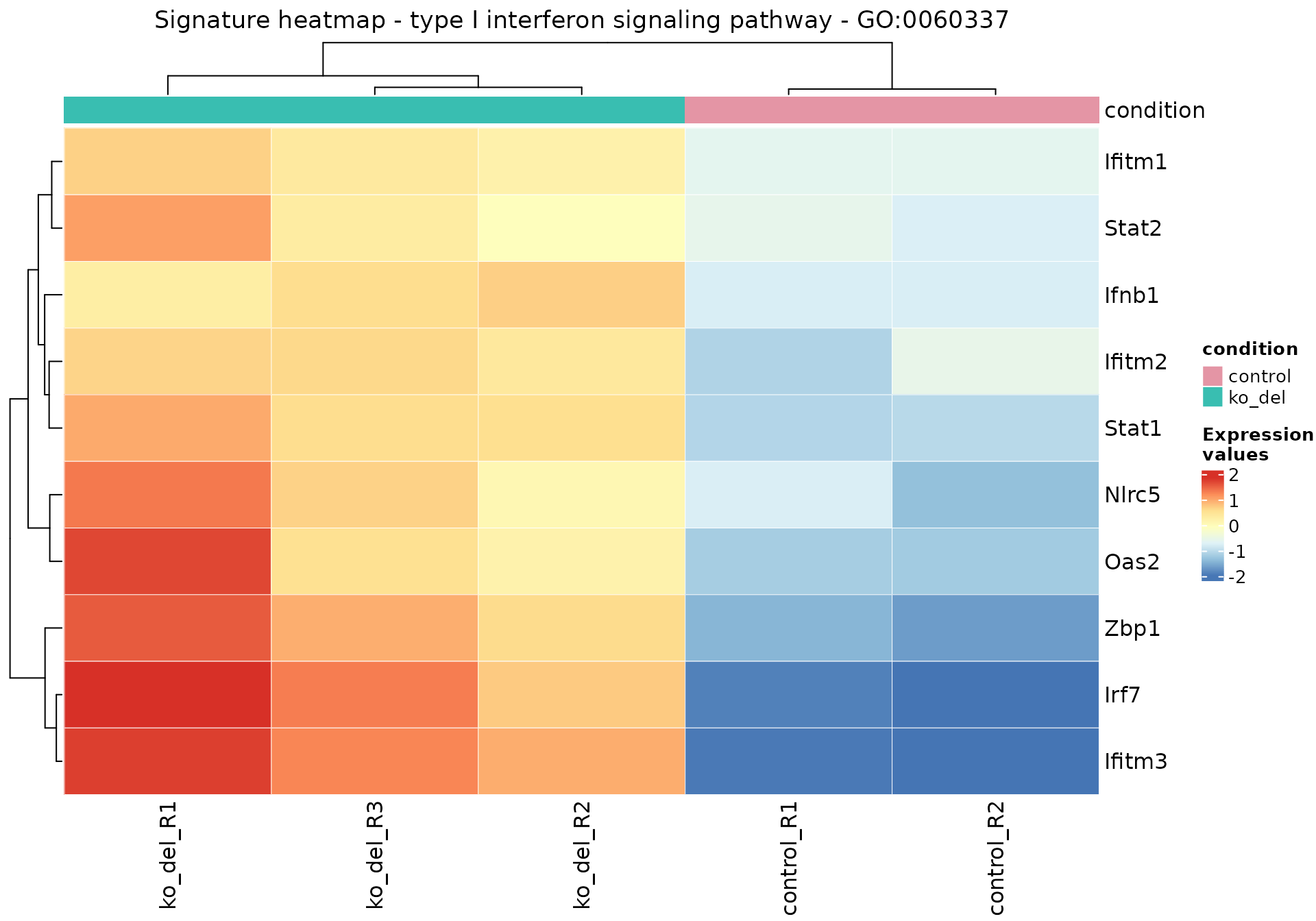
go_2_html("GO:0060337",
  res_enrich = res_enrich_a20
)
GO ID: GO:0060337
Term: type I interferon signaling pathway
p-value: 6e-05
Z-score: 3.16
Aggregated score: 3.74
Ontology: BP
Definition: A series of molecular signals initiated by the binding of a type I interferon to a receptor on the surface of a cell, and ending with regulation of a downstream cellular process, e.g. transcription. Type I interferons include the interferon-alpha, beta, delta, episilon, zeta, kappa, tau, and omega gene families.
Synonym: type I interferon-activated signaling pathway
Synonym: type I interferon-mediated signalling pathway
Synonym: type I interferon-mediated signaling pathway
signature_volcano(
  gtl = gtl_alma,
  geneset_id = "GO:0060337",
  FDR = 0.05,
  color = "#1a81c2"
)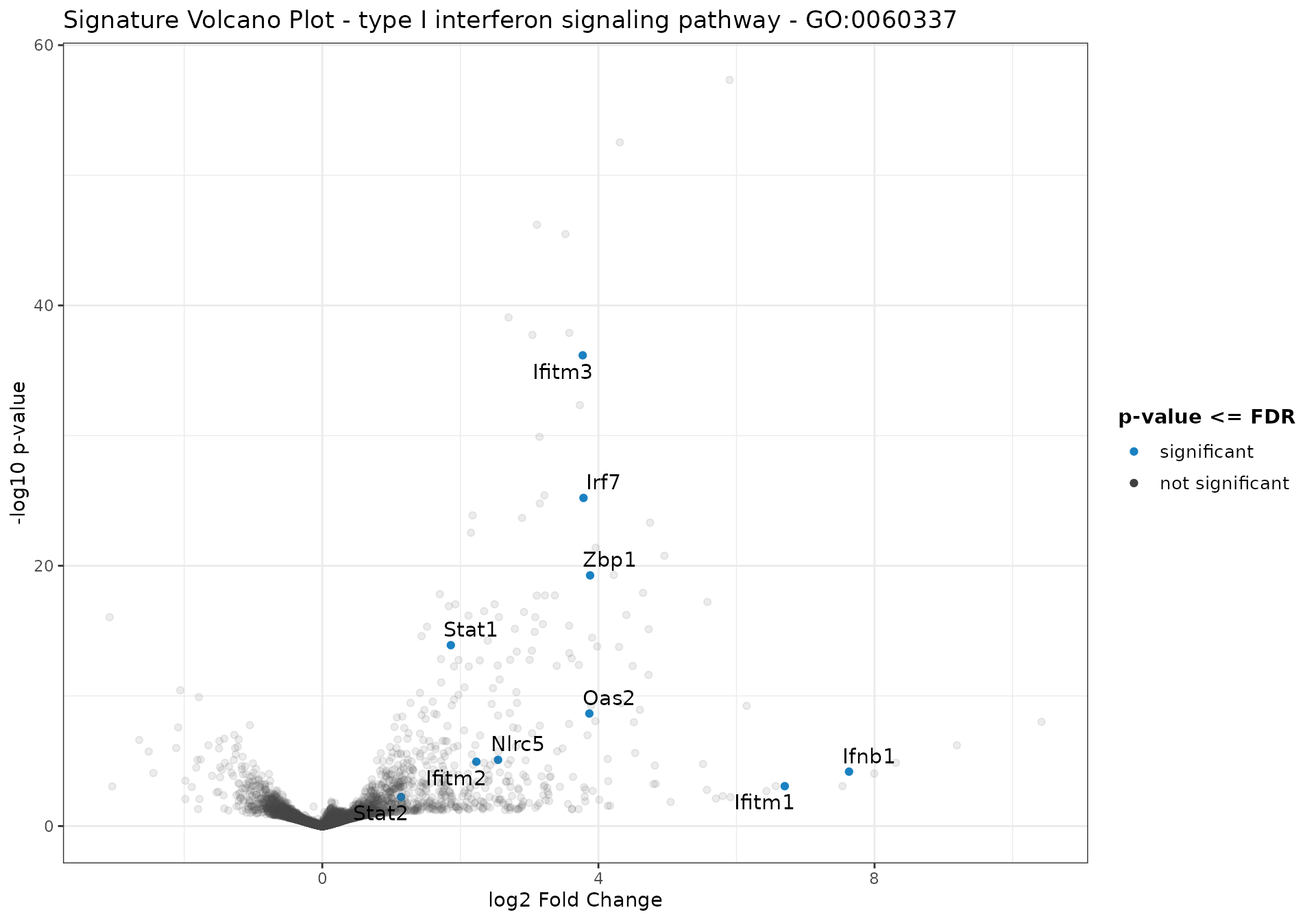
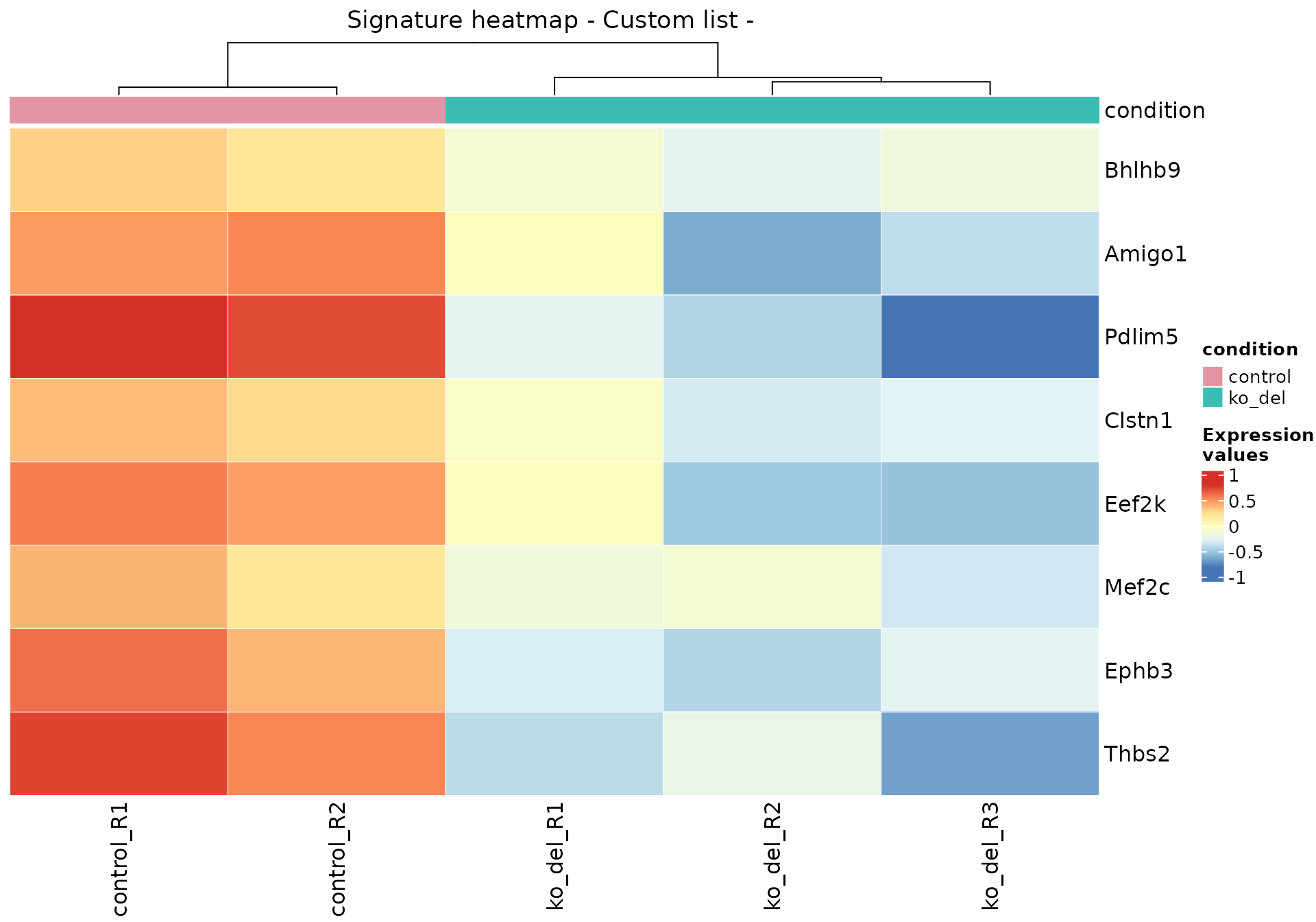
As an example, these plots are related to the data presented in Figure 3 of (Mohebiany et al. 2020).
genes_synapse_assembly <- c(
  "Bhlhb9",
  "Mef2c",
  "Clstn1",
  "Amigo1",
  "Eef2k",
  "Ephb3",
  "Thbs2",
  "Pdlim5"
)

genes_synapse_assembly_ensids <-
  anno_df$gene_id[match(genes_synapse_assembly, anno_df$gene_name)]

gs_heatmap(
  se = vst_alma,
  gtl = gtl_alma,
  genelist = genes_synapse_assembly_ensids,
  cluster_columns = TRUE,
  cluster_rows = FALSE,
  anno_col_info = "condition"
)
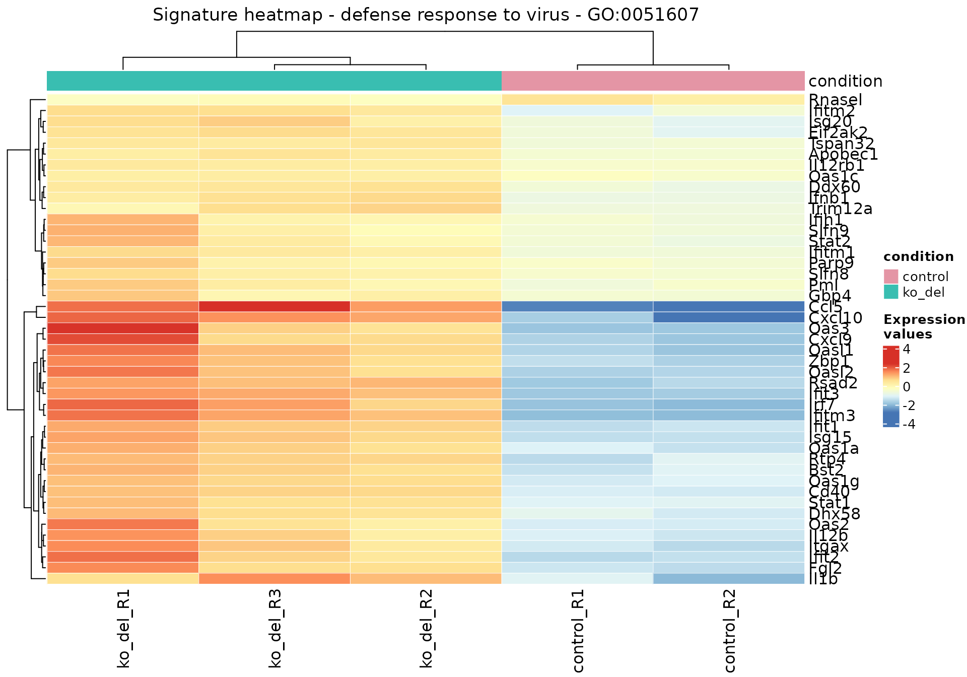
res_enrich_a20[res_enrich_a20$gs_id == "GO:0051607", ]
#>                 gs_id            gs_description gs_pvalue
#> GO:0051607 GO:0051607 defense response to virus   3.1e-13
#>                                                                                                                                                                                                                                                                                   gs_genes
#> GO:0051607 Apobec1,Bst2,Ccl5,Cd40,Cxcl10,Cxcl9,Ddx60,Dhx58,Eif2ak2,Fgl2,Gbp4,Ifih1,Ifit1,Ifit2,Ifit3,Ifitm1,Ifitm2,Ifitm3,Ifnb1,Il12b,Il12rb1,Il1b,Irf7,Isg15,Isg20,Itgax,Oas1a,Oas1c,Oas1g,Oas2,Oas3,Oasl1,Oasl2,Parp9,Pml,Rnasel,Rsad2,Rtp4,Slfn8,Slfn9,Stat1,Stat2,Trim12a,Tspan32,Zbp1
#>            gs_de_count gs_bg_count Expected DE_count  z_score aggr_score
#> GO:0051607          45         198    11.94       45 6.410062   2.939613

gs_heatmap(
  se = vst_alma,
  gtl = gtl_alma,
  geneset_id = "GO:0051607",
  cluster_columns = TRUE,
  anno_col_info = "condition"
)
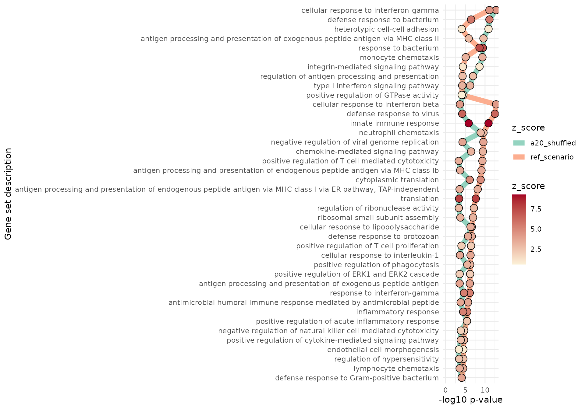
Comparing enrichment results
Imagine we were to compare the enrichment results from our study to another one where the same set of pathways is reported - or alternatively, on the same dataset but focusing on a different contrast. We can replicate such a situation by shuffling the results in res_enrich_a20, and displaying the comparison with gs_radar(), gs_summary_overview_pair(), or gs_horizon()
# with more than one set
res_enrich_shuffled <- res_enrich_a20[1:60, ]
set.seed(42)
shuffled_ones <- sample(seq_len(60)) # to generate permuted p-values
res_enrich_shuffled$gs_pvalue <- res_enrich_shuffled$gs_pvalue[shuffled_ones]
# ideally, I would also permute the z scores and aggregated scores
gs_radar(res_enrich = res_enrich_a20,
         res_enrich2 = res_enrich_shuffled)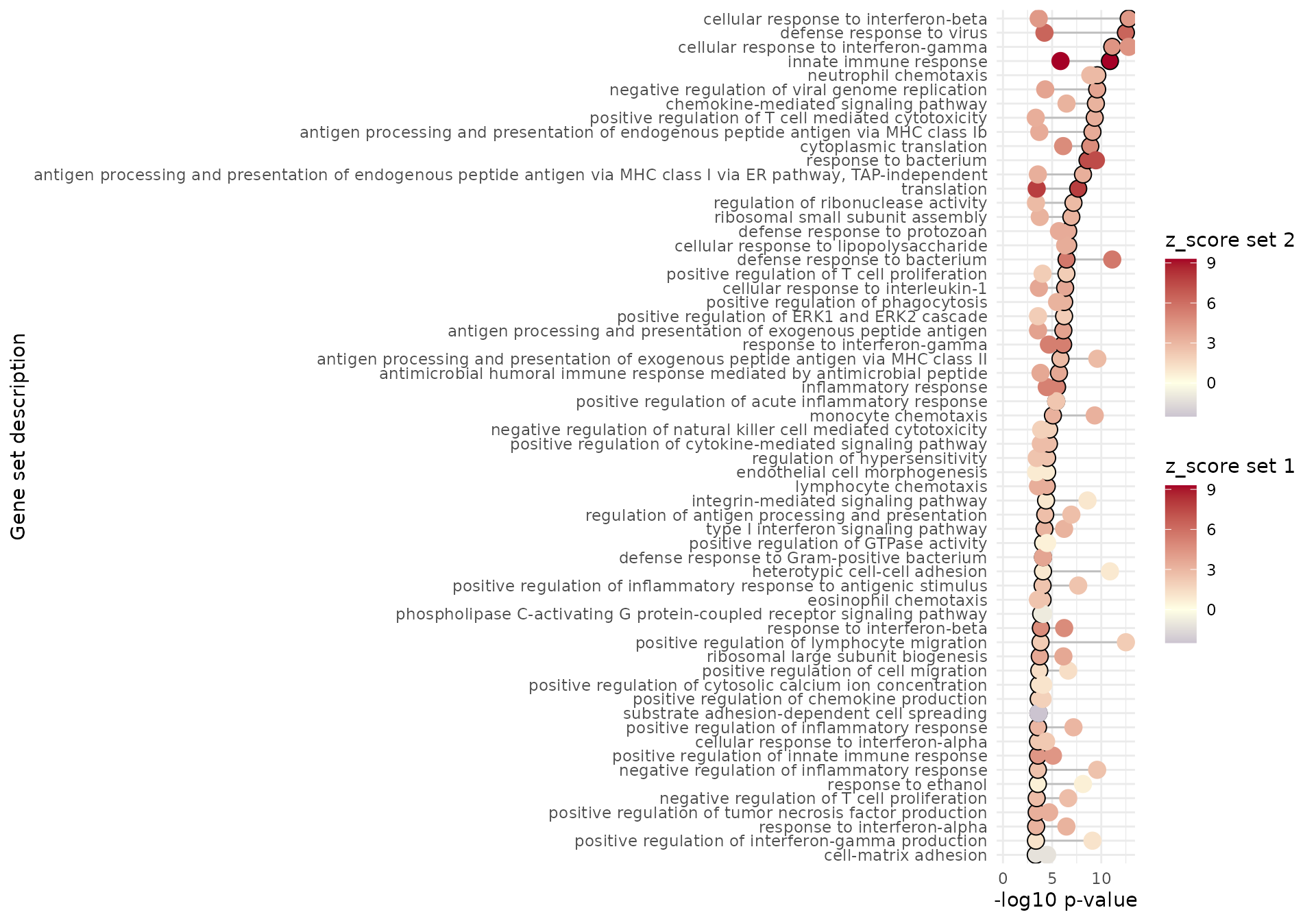
gs_horizon(res_enrich = res_enrich_a20,
           compared_res_enrich_list = list(
             a20_shuffled = res_enrich_shuffled),
           n_gs = 40
          )
Integrated reporting
The reporting functionality of happy_hour() can be called anytime also from the command line, focusing on a subset of genes and genesets of interest, which will be presented with additional detail in the output document.
happy_hour(
  gtl = gtl_alma,
  project_id = "a20-microglia",
  mygenesets = c(
    res_enrich_a20$gs_id[c(1:5, 11, 31)],
    # additionally selecting some by id
    "GO:0051963" # regulation of synapse assembly
  ),
  mygenes = c(
    "ENSMUSG00000035042",
    "ENSMUSG00000074896",
    "ENSMUSG00000035929"
  ),
  open_after_creating = TRUE
)
Alternate entry point - using edgeR for the DE analysis
It is also possible to use edgeR to perform the steps before using GeneTonic.
The chunk below reports an example of how to do so - imagine you start with a DGE object called dge_alma:
library("DEFormats")
library("edgeR")
dge_alma <- as.DGEList(dds_alma)
We add the gene symbols for ease of readability…
… and perform a QL-based analysis, obtaining the qlf object at the end of it.
keep <- filterByExpr(dge_alma)
table(keep)
#> keep
#> FALSE  TRUE
#> 29148 12240
y <- dge_alma[keep, , keep.lib.sizes = FALSE]
y <- calcNormFactors(y)
conds <- dge_alma$samples$group
design <- model.matrix(~conds)
y <- estimateDisp(y, design)
# To perform quasi-likelihood F-tests:
fit <- glmQLFit(y, design)
qlf <- glmQLFTest(fit, coef = "condsko_del")
plotMD(qlf)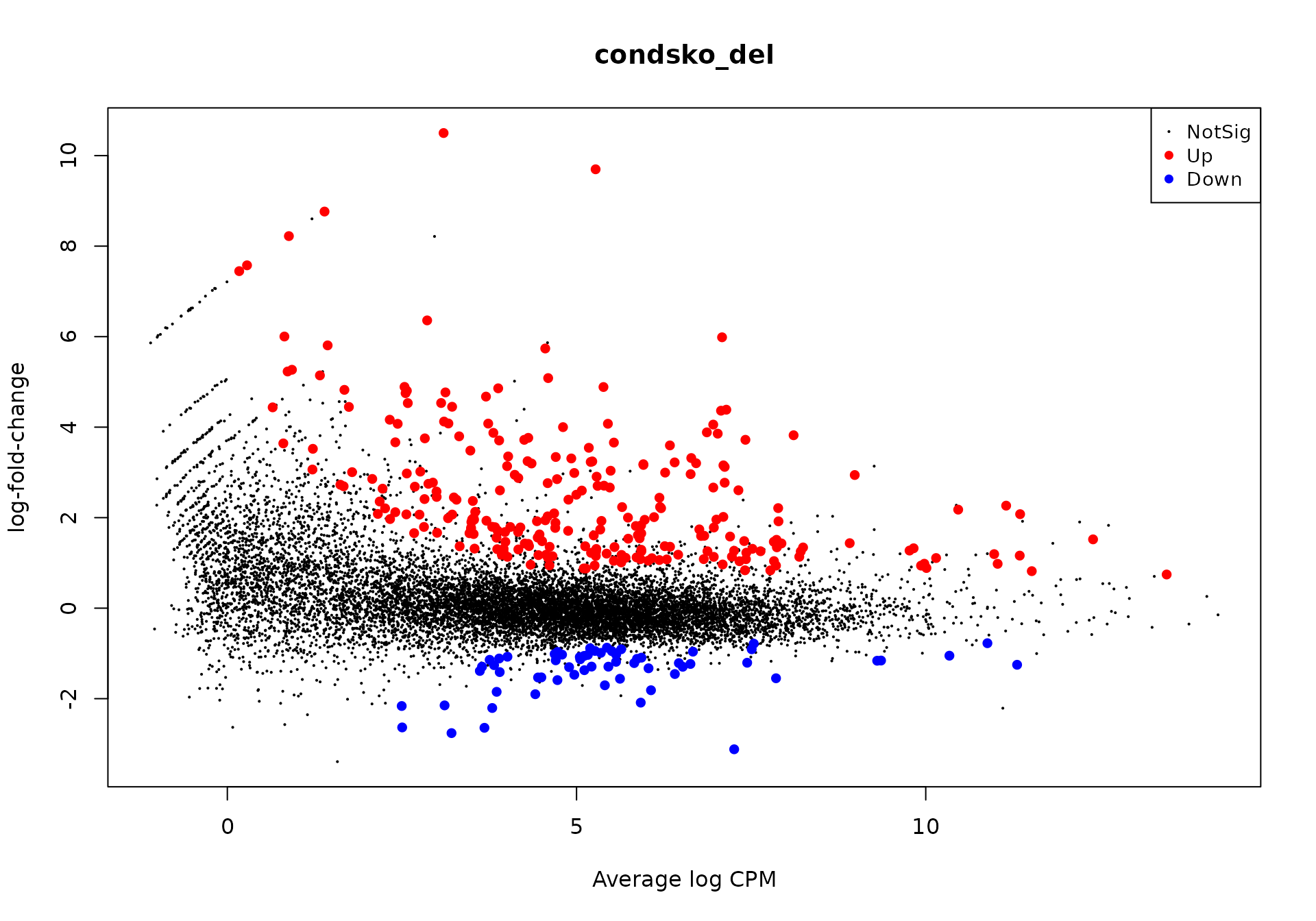
We would need to convert these objects back to the DESeq2-based objects.
convert_to_DESeqResults <- function(dgelrt, dge, FDR = 0.05) {
  tbledger <- as.data.frame(topTags(dgelrt, n = Inf))
  colnames(tbledger)[colnames(tbledger) == "PValue"] <- "pvalue"
  colnames(tbledger)[colnames(tbledger) == "logFC"] <- "log2FoldChange"
  colnames(tbledger)[colnames(tbledger) == "logCPM"] <- "baseMean"
  colnames(tbledger)[colnames(tbledger) == "SYMBOL"] <- "SYMBOL"

  # get from the logCPM to something on the scale of the baseMean
  tbledger$baseMean <- (2^tbledger$baseMean) * mean(dge$samples$lib.size) / 1e6

  # use the constructor for DESeqResults
  edger_resu <- DESeqResults(DataFrame(tbledger))
  edger_resu <- DESeq2:::pvalueAdjustment(edger_resu,
    independentFiltering = FALSE,
    alpha = FDR, pAdjustMethod = "BH"
  )
}

res_de_from_edgeR <- convert_to_DESeqResults(qlf, dge_alma)

summary(decideTestsDGE(qlf))
#>        condsko_del
#> Down            62
#> NotSig       11923
#> Up             255
summary(res_de_from_edgeR, alpha = 0.05)
#>
#> out of 12240 with nonzero total read count
#> adjusted p-value < 0.05
#> LFC > 0 (up)       : 255, 2.1%
#> LFC < 0 (down)     : 62, 0.51%
#> outliers [1]       : 0, 0%
#> low counts [2]     : 0, 0%
#> (mean count < 0)
#> [1] see 'cooksCutoff' argument of ?results
#> [2] see 'independentFiltering' argument of ?results

dds_alma_from_edgeR <- as.DESeqDataSet(dge_alma)
Imagine we have already our res_enrich object, obtained in any of the ways specified above - then we can simply launch GeneTonic with these commands (utilizing the anno_df object from the examples above):
gtl_from_edgeR <- GeneTonic_list(
  dds = dds_alma_from_edgeR,
  res_de = res_de_from_edgeR,
  res_enrich = res_enrich_clusterprofiler,
  annotation_obj = anno_df
)
GeneTonic(gtl = gtl_from_edgeR)
Session information
sessionInfo()
#> R version 4.1.1 (2021-08-10)
#> Platform: x86_64-pc-linux-gnu (64-bit)
#> Running under: Ubuntu 20.04.3 LTS
#>
#> Matrix products: default
#> BLAS/LAPACK: /usr/lib/x86_64-linux-gnu/openblas-pthread/libopenblasp-r0.3.8.so
#>
#> locale:
#>  [1] LC_CTYPE=en_US.UTF-8       LC_NUMERIC=C
#>  [3] LC_TIME=en_US.UTF-8        LC_COLLATE=en_US.UTF-8
#>  [5] LC_MONETARY=en_US.UTF-8    LC_MESSAGES=C
#>  [7] LC_PAPER=en_US.UTF-8       LC_NAME=C
#>  [9] LC_ADDRESS=C               LC_TELEPHONE=C
#> [11] LC_MEASUREMENT=en_US.UTF-8 LC_IDENTIFICATION=C
#>
#> attached base packages:
#> [1] stats4    stats     graphics  grDevices utils     datasets  methods
#> [8] base
#>
#> other attached packages:
#>  [1] edgeR_3.35.1                limma_3.49.4
#>  [3] DEFormats_1.21.0            magrittr_2.0.1
#>  [5] visNetwork_2.1.0            apeglm_1.15.0
#>  [7] GeneTonic_1.5.6             DT_0.19
#>  [9] ideal_1.17.4                pcaExplorer_2.19.1
#> [11] org.Mm.eg.db_3.14.0         pheatmap_1.0.12
#> [13] topGO_2.45.0                SparseM_1.81
#> [15] GO.db_3.14.0                AnnotationDbi_1.55.1
#> [17] graph_1.71.2                DESeq2_1.33.5
#> [19] SummarizedExperiment_1.23.5 Biobase_2.53.0
#> [21] MatrixGenerics_1.5.4        matrixStats_0.61.0
#> [23] GenomicRanges_1.45.0        GenomeInfoDb_1.29.8
#> [25] IRanges_2.27.2              S4Vectors_0.31.5
#> [27] BiocGenerics_0.39.2         GeneTonicWorkshop_0.9.0
#>
#> loaded via a namespace (and not attached):
#>   [1] rappdirs_0.3.3           rtracklayer_1.53.1       AnnotationForge_1.35.2
#>   [4] coda_0.19-4              ragg_1.1.3               pkgmaker_0.32.2
#>   [7] tidyr_1.1.4              ggplot2_3.3.5            bit64_4.0.5
#>  [10] knitr_1.36               DelayedArray_0.19.4      data.table_1.14.2
#>  [13] KEGGREST_1.33.0          RCurl_1.98-1.5           doParallel_1.0.16
#>  [16] generics_0.1.0           GenomicFeatures_1.45.2   RSQLite_2.2.8
#>  [19] bit_4.0.4                webshot_0.5.2            xml2_1.3.2
#>  [22] httpuv_1.6.3             assertthat_0.2.1         viridis_0.6.2
#>  [25] xfun_0.27                hms_1.1.1                jquerylib_0.1.4
#>  [28] evaluate_0.14            promises_1.2.0.1         IHW_1.21.1
#>  [31] TSP_1.1-11               fansi_0.5.0              restfulr_0.0.13
#>  [34] progress_1.2.2           caTools_1.18.2           dendextend_1.15.1
#>  [37] dbplyr_2.1.1             Rgraphviz_2.37.2         igraph_1.2.7
#>  [40] DBI_1.1.1                geneplotter_1.71.0       htmlwidgets_1.5.4
#>  [43] purrr_0.3.4              ellipsis_0.3.2           crosstalk_1.1.1
#>  [46] backports_1.2.1          dplyr_1.0.7              bookdown_0.24
#>  [49] annotate_1.71.0          gridBase_0.4-7           biomaRt_2.49.6
#>  [52] vctrs_0.3.8              cachem_1.0.6             withr_2.4.2
#>  [55] ggforce_0.3.3            checkmate_2.0.0          bdsmatrix_1.3-4
#>  [58] GenomicAlignments_1.29.0 fdrtool_1.2.16           prettyunits_1.1.1
#>  [61] cluster_2.1.2            backbone_1.5.1           lazyeval_0.2.2
#>  [64] crayon_1.4.1             genefilter_1.75.1        pkgconfig_2.0.3
#>  [67] slam_0.1-48              labeling_0.4.2           tweenr_1.0.2
#>  [70] nlme_3.1-153             seriation_1.3.1          rlang_0.4.12
#>  [73] lifecycle_1.0.1          miniUI_0.1.1.1           colourpicker_1.1.1
#>  [76] registry_0.5-1           filelock_1.0.2           BiocFileCache_2.1.1
#>  [79] GOstats_2.59.1           rprojroot_2.0.2          polyclip_1.10-0
#>  [82] rngtools_1.5.2           Matrix_1.3-4             lpsymphony_1.21.0
#>  [85] base64enc_0.1-3          geneLenDataBase_1.29.0   GlobalOptions_0.1.2
#>  [88] png_0.1-7                viridisLite_0.4.0        rjson_0.2.20
#>  [91] bitops_1.0-7             shinydashboard_0.7.2     KernSmooth_2.23-20
#>  [94] Biostrings_2.61.2        blob_1.2.2               shape_1.4.6
#>  [97] rintrojs_0.3.0           stringr_1.4.0            shinyAce_0.4.1
#> [100] scales_1.1.1             memoise_2.0.0            GSEABase_1.55.1
#> [103] plyr_1.8.6               gplots_3.1.1             zlibbioc_1.39.0
#> [106] threejs_0.3.3            compiler_4.1.1           bbmle_1.0.24
#> [109] BiocIO_1.3.0             RColorBrewer_1.1-2       clue_0.3-60
#> [112] Rsamtools_2.9.1          XVector_0.33.0           Category_2.59.0
#> [115] MASS_7.3-54              mgcv_1.8-38              tidyselect_1.1.1
#> [118] stringi_1.7.5            textshaping_0.3.6        shinyBS_0.61
#> [121] highr_0.9                emdbook_1.3.12           yaml_2.2.1
#> [124] locfit_1.5-9.4           ggrepel_0.9.1            grid_4.1.1
#> [127] sass_0.4.0               tools_4.1.1              parallel_4.1.1
#> [130] circlize_0.4.13          foreach_1.5.1            gridExtra_2.3
#> [133] farver_2.1.0             digest_0.6.28            shiny_1.7.1
#> [136] Rcpp_1.0.7               later_1.3.0              shinyWidgets_0.6.2
#> [139] httr_1.4.2               ComplexHeatmap_2.9.4     colorspace_2.0-2
#> [142] XML_3.99-0.8             fs_1.5.0                 splines_4.1.1
#> [145] tippy_0.1.0              RBGL_1.69.0              expm_0.999-6
#> [148] pkgdown_1.6.1            plotly_4.10.0            systemfonts_1.0.3
#> [151] xtable_1.8-4             jsonlite_1.7.2           heatmaply_1.3.0
#> [154] dynamicTreeCut_1.63-1    UpSetR_1.4.0             R6_2.5.1
#> [157] pillar_1.6.4             htmltools_0.5.2          mime_0.12
#> [160] NMF_0.23.0               glue_1.4.2               fastmap_1.1.0
#> [163] BiocParallel_1.27.17     bs4Dash_2.0.3            codetools_0.2-18
#> [166] mvtnorm_1.1-3            utf8_1.2.2               lattice_0.20-45
#> [169] bslib_0.3.1              tibble_3.1.5             numDeriv_2016.8-1.1
#> [172] curl_4.3.2               BiasedUrn_1.07           rentrez_1.2.3
#> [175] gtools_3.9.2             survival_3.2-13          rmarkdown_2.11
#> [178] desc_1.4.0               munsell_0.5.0            GetoptLong_1.0.5
#> [181] GenomeInfoDbData_1.2.7   iterators_1.0.13         goseq_1.45.0
#> [184] reshape2_1.4.4           gtable_0.3.0             shinycssloaders_1.0.0