Visually enhances a functional enrichment result table

Creates a visual summary for the results of a functional enrichment analysis, by displaying also the components of each gene set and their expression change in the contrast of interest

enhance_table(
  res_enrich,
  res_de,
  annotation_obj,
  gtl = NULL,
  n_gs = 50,
  gs_ids = NULL,
  chars_limit = 70,
  plot_style = c("point", "ridgeline"),
  ridge_color = c("gs_id", "gs_score"),
  plot_title = NULL
)

Arguments

res_enrich

A data.frame object, storing the result of the functional enrichment analysis. See more in the main function, GeneTonic(), to check the formatting requirements (a minimal set of columns should be present).

res_de

A DESeqResults object.

annotation_obj

A data.frame object with the feature annotation. information, with at least two columns, gene_id and gene_name.

gtl

A GeneTonic-list object, containing in its slots the arguments specified above: dds, res_de, res_enrich, and annotation_obj - the names of the list must be specified following the content they are expecting

n_gs

Integer value, corresponding to the maximal number of gene sets to be displayed.

gs_ids

Character vector, containing a subset of gs_id as they are available in res_enrich. Lists the gene sets to be displayed.

chars_limit

Integer, number of characters to be displayed for each geneset name.

plot_style

Character value, one of "point" or "ridgeline". Defines the style of the plot to summarize visually the table.

ridge_color

Character value, one of "gs_id" or "gs_score", controls the fill color of the ridge lines. If selecting "gs_score", the z_score column must be present in the enrichment results table - see get_aggrscores() to do that.

plot_title

Character string, used as title for the plot. If left NULL, it defaults to a general description of the plot and of the DE contrast.

Value

A ggplot object

Examples

library("macrophage")
library("DESeq2")
library("org.Hs.eg.db")
library("AnnotationDbi")

# dds object
data("gse", package = "macrophage")
dds_macrophage <- DESeqDataSet(gse, design = ~ line + condition)
#> using counts and average transcript lengths from tximeta
rownames(dds_macrophage) <- substr(rownames(dds_macrophage), 1, 15)
dds_macrophage <- estimateSizeFactors(dds_macrophage)
#> using 'avgTxLength' from assays(dds), correcting for library size

# annotation object
anno_df <- data.frame(
  gene_id = rownames(dds_macrophage),
  gene_name = mapIds(org.Hs.eg.db,
    keys = rownames(dds_macrophage),
    column = "SYMBOL",
    keytype = "ENSEMBL"
  ),
  stringsAsFactors = FALSE,
  row.names = rownames(dds_macrophage)
)
#> 'select()' returned 1:many mapping between keys and columns

# res object
data(res_de_macrophage, package = "GeneTonic")
res_de <- res_macrophage_IFNg_vs_naive

# res_enrich object
data(res_enrich_macrophage, package = "GeneTonic")
res_enrich <- shake_topGOtableResult(topgoDE_macrophage_IFNg_vs_naive)
#> Found 500 gene sets in `topGOtableResult` object.
#> Converting for usage in GeneTonic...
res_enrich <- get_aggrscores(res_enrich, res_de, anno_df)
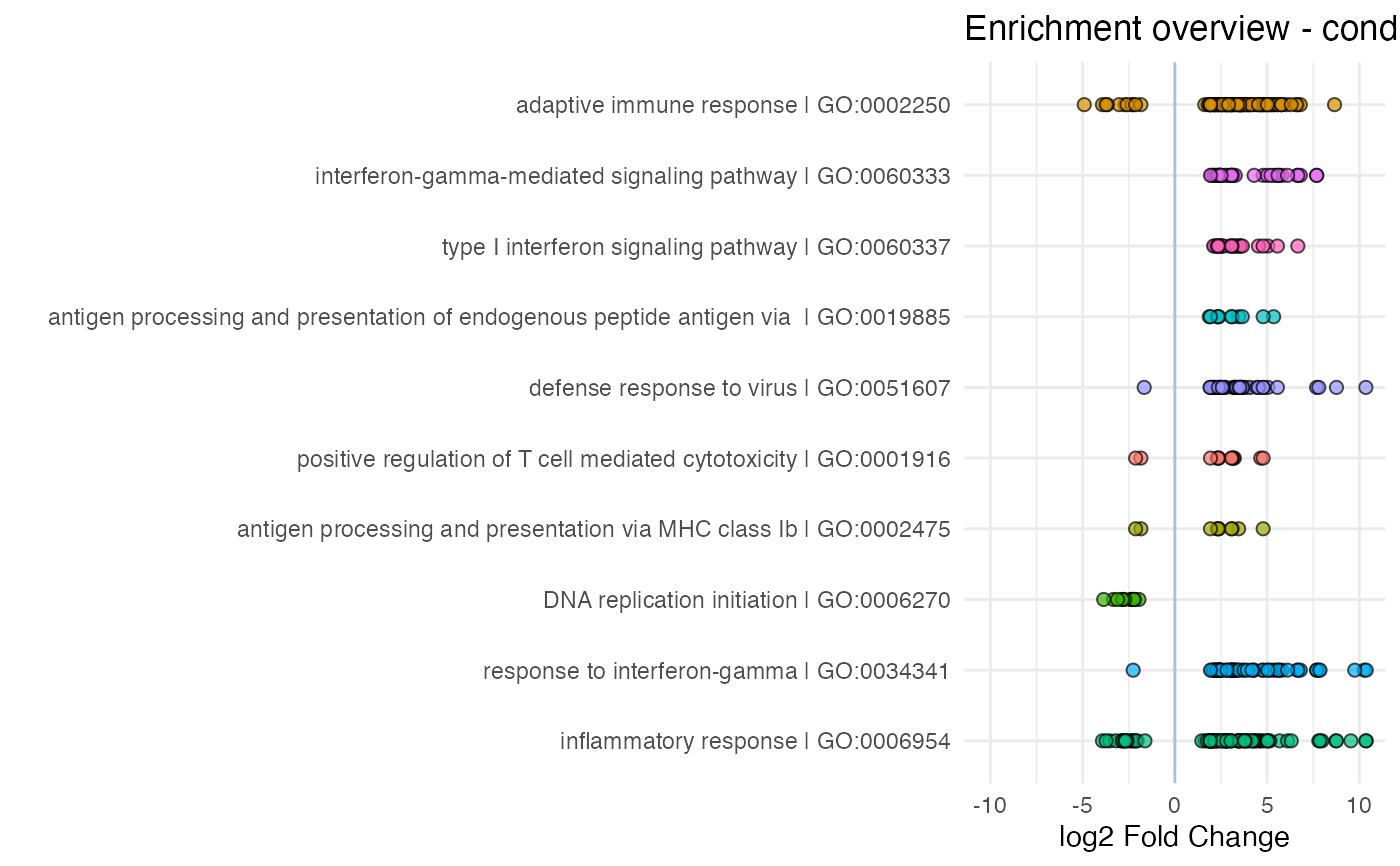
enhance_table(res_enrich,
  res_de,
  anno_df,
  n_gs = 10
)


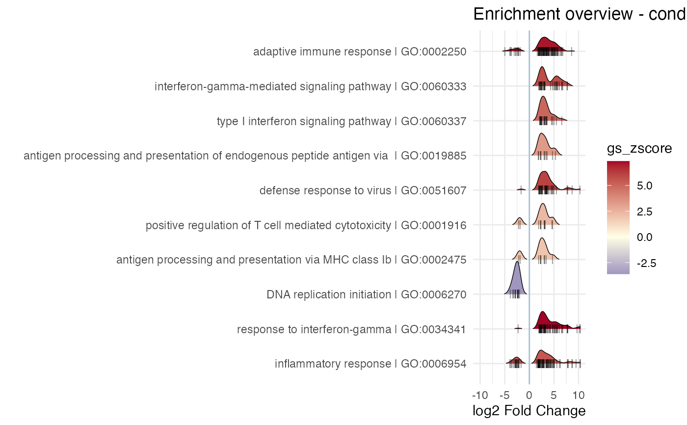
# using the ridge line as a style, also coloring by the Z score
res_enrich_withscores <- get_aggrscores(
  res_enrich,
  res_de,
  anno_df
)
enhance_table(res_enrich_withscores,
  res_de,
  anno_df,
  n_gs = 10, 
  plot_style = "ridgeline",
  ridge_color = "gs_score"
)
#> Picking joint bandwidth of 0.553