Plot expression values for a gene — gene

Plot expression values (e.g. normalized counts) for a gene of interest, grouped by experimental group(s) of interest

gene_plot(
  dds,
  gene,
  intgroup = "condition",
  assay = "counts",
  annotation_obj = NULL,
  normalized = TRUE,
  transform = TRUE,
  labels_display = TRUE,
  labels_repel = TRUE,
  plot_type = "auto",
  return_data = FALSE,
  gtl = NULL
)

Arguments

dds: A DESeqDataSet object, normally obtained after running your data through the DESeq2 framework.
gene: Character, specifies the identifier of the feature (gene) to be plotted
intgroup: A character vector of names in colData(dds) to use for grouping. Note: the vector components should be categorical variables.
assay: Character, specifies with assay of the dds object to use for reading out the expression values. Defaults to "counts".
annotation_obj: A data.frame object with the feature annotation information, with at least two columns, gene_id and gene_name.
normalized: Logical value, whether the expression values should be normalized by their size factor. Defaults to TRUE, applies when assay is "counts"
transform: Logical value, corresponding whether to have log scale y-axis or not. Defaults to TRUE.
labels_display: Logical value. Whether to display the labels of samples, defaults to TRUE.
labels_repel: Logical value. Whether to use ggrepel's functions to place labels; defaults to TRUE
plot_type: Character, one of "auto", "jitteronly", "boxplot", "violin", or "sina". Defines the type of geom_ to be used for plotting. Defaults to auto, which in turn chooses one of the layers according to the number of samples in the smallest group defined via intgroup
return_data: Logical, whether the function should just return the data.frame of expression values and covariates for custom plotting. Defaults to FALSE.
gtl: A GeneTonic-list object, containing in its slots the arguments specified above: dds, res_de, res_enrich, and annotation_obj - the names of the list must be specified following the content they are expecting

Value

A ggplot object

Details

The result of this function can be fed directly to plotly::ggplotly() for interactive visualization, instead of the static ggplot viz.

Examples

library("macrophage")
library("DESeq2")
library("org.Hs.eg.db")

# dds object
data("gse", package = "macrophage")
dds_macrophage <- DESeqDataSet(gse, design = ~ line + condition)
#> using counts and average transcript lengths from tximeta
rownames(dds_macrophage) <- substr(rownames(dds_macrophage), 1, 15)
dds_macrophage <- estimateSizeFactors(dds_macrophage)
#> using 'avgTxLength' from assays(dds), correcting for library size

# annotation object
anno_df <- data.frame(
  gene_id = rownames(dds_macrophage),
  gene_name = mapIds(org.Hs.eg.db,
    keys = rownames(dds_macrophage),
    column = "SYMBOL",
    keytype = "ENSEMBL"
  ),
  stringsAsFactors = FALSE,
  row.names = rownames(dds_macrophage)
)
#> 'select()' returned 1:many mapping between keys and columns

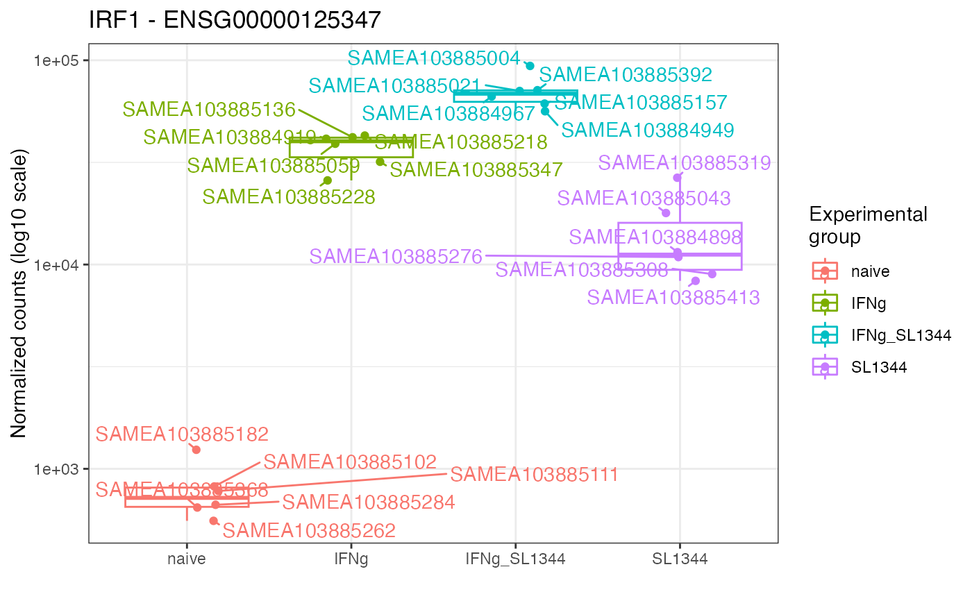
gene_plot(dds_macrophage,
  gene = "ENSG00000125347",
  intgroup = "condition",
  annotation_obj = anno_df
)